深入理解word2vec

How to represent meanings?

如何在数学上表达词义？

Vector space models (VSMs) 表示把单词映射到(嵌入)连续的矢量空间, 而且理论上语义相似的单词会映射到空间中临近的位置。VSMs是一个历史悠久的NLP理论，但所有实现方法都不同程度依赖于Distributional Hypothesis, 即出现在相同（相似）的上下文中的单词具有相同（相似）的语义意义。利用此原则的方法大致可以分为两类: Count-based methods (例如, Latent Semantic Analysis))和Predictive models(例如 neural net language models (NNLM))。

具体的区别详见Baroni et al.. 但总的来说，Count-based methods 统计词汇间的共现频率，然后把co-occurs matrix 映射到向量空间中；而Predictive models直接通过上下文预测单词的方式来学习向量空间（也就是模型参数空间）。

Word2vec 是一种计算特别高效的predictive model, 用于从文本中学习word embeddings。它有两种方案, Continuous Bag-of-Words model (CBOW) 和 Skip-Gram model (Section 3.1 and 3.2 in Mikolov et al.).

从算法上讲, 两种方案是相似的, 只不过 CBOW 会从source context-words ('the cat sits on the')预测目标单词(例如"mat"); 而skip-gram则相反, 预测目标单词的source context-words。Skip-gram这种做法可能看起来有点随意. 但从统计上看, CBOW 会平滑大量分布信息(通过将整个上下文视为一个观测值), 在大多数情况下, 这对较小的数据集是很有用的。但是, Skip-gram将每个context-target pair视为新的观测值, 当数据集较大时, 这往往带来更好的效果。

Word2vec的算法流程是：

Start with a sentence: “the quick brown fox jumps.”
Use a sliding window across the sentence to create (context, target) pairs, where the target is the center word, and the context is the surrounding words:

([the, brown], quick)
([quick, fox], brown)
([brown, jumps], fox)

Use a lookup embedding layer to convert the context words into vectors, and average them to get a single input vector that represents the full context.
Using the context vector as input into a fully connected Neural Network layer with a Softmax transformation. This results in a probability for every word in your entire vocabulary for being the correct target given the current context.
Minimize the cross-entropy loss where label = 1 for the correct target word, and label = 0 for all other words.

优化目标函数

NNLM 的训练是利用最大似然 maximum likelihood (ML) 原则来最大化给定上文单词$h$ (for “history”) 预测下一个词的概率 $w_t$ (for “target”)。

$$ \begin{align} P(w_t | h) &= \text{softmax}(\text{score}(w_t, h)) \\ &= \frac{\exp { \text{score}(w_t, h) } } {\sum_\text{Word w’ in Vocab} \exp { \text{score}(w’, h) } } \end{align} $$

其中 $\text{score}(w_t, h)$ 计算 word $w_t$ 和 context $h$ 的相关性 (一般用点乘).

训练时，最大化

$$ \begin{align} J_\text{ML} &= \log P(w_t | h) \\ &= \text{score}(w_t, h) - \log \left( \sum_\text{Word w’ in Vocab} \exp { \text{score}(w’, h) } \right). \end{align} $$

这么计算成本很高，因为在每一训练步，需要为词汇表 $V$ 中的每一个词汇 $w’$ 计算在当前上下文 $h$ 的分数概率。

Negative sampling

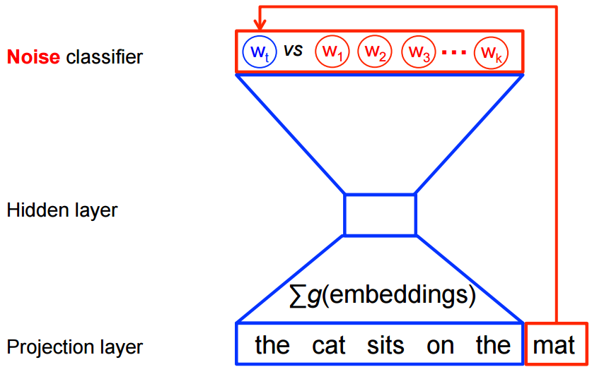
但是，word2vec的目的是特征学习，而不是学习完整的概率语言模型。所以word2vec（CBOW和Skip gram一样）的训练目标函数其实是一个二分类模型(logistic regression)，给定一个上下文，在 $k$ 个噪声词（根据算法选出）和一个真正的目标词汇$w_t$中识别出目标词$w_t$。如下图(以CBOW为例, Skip gram方向反过来)

目标函数变为最大化: $$ J_\text{NEG} = \log Q_\theta(D=1 |w_t, h) + k \mathop{\mathbb{E}}{\tilde w \sim P_n} \left[ \log Q\theta(D = 0 |\tilde w, h) \right] $$

where $Q_\theta(D=1 | w, h)$ is the binary logistic regression probability under the model of seeing the word $w$ in the context $h$ in the dataset $D$, calculated in terms of the learned embedding vectors $\theta$. In practice we approximate the expectation by drawing $k$ contrastive words from the noise distribution (i.e. we compute a Monte Carlo average).

负采样是指每个训练样本仅更新模型权重的一小部分：

负采样的选择是基于 unigram 分布 $f(w_i)$: 一个词作为负面样本被选择的概率与其出现的频率有关，更频繁的词更可能被选作负面样本。 $$ P(w_i) = \frac{ {f(w_i)}^{3/4} }{\sum_{j=0}^{n}\left( {f(w_j)}^{3/4} \right) } $$ 负采样带来的好处是

训练速度不再受限于 vocabulary size
能够并行实现
模型的表现更好。因为负采样契合NLP的稀疏性质，大部分情况下，虽然语料库很大，但是每一个词只跟很小部分词由关联，大部分词之间是毫无关联的，从无关联的两个词之间也别指望能学到什么有用的信息，不如直接忽略。模型的表现更好。因为负采样契合NLP的稀疏性质，大部分情况下，虽然语料库很大，但是每一个词只跟很小部分词由关联，大部分词之间是毫无关联的，从无关联的两个词之间也别指望能学到什么有用的信息，不如直接忽略。
通过这种方式把学习P分布的无监督学习任务改造为监督学习。

每个词由两个向量表示：

$v_w$, 表示这个词作为中心词 (Focus Word) 时的样子。
$u_w$, 表示它作为另一个中心词的上下文 (Context Word) 时的样子。

这样, 对于一个中心词 $c$ 和外围词$o$: $$ P(o|c) = \frac{exp(u^T_o v_c)}{\sum_{w \in V} \left( {exp(u^T_w v_c)} \right)} $$

在C语言的源代码里，这些向量由两个数组 (Array) 分别负责： syn0数组，负责某个词作为中心词时的向量。是随机初始化的。

// https://github.com/tmikolov/word2vec/blob/20c129af10659f7c50e86e3be406df663beff438/word2vec.c#L369
for (a = 0; a < vocab_size; a++) for (b = 0; b < layer1_size; b++) {
     next_random = next_random * (unsigned long long)25214903917 + 11;
     syn0[a * layer1_size + b] =
        (((next_random & 0xFFFF) / (real)65536) - 0.5) / layer1_size;
   }

syn1neg数组，负责这个词作为上下文时的向量。是零初始化的。

// https://github.com/tmikolov/word2vec/blob/20c129af10659f7c50e86e3be406df663beff438/word2vec.c#L365
for (a = 0; a < vocab_size; a++) for (b = 0; b < layer1_size; b++)
   syn1neg[a * layer1_size + b] = 0;

训练时，先选出一个中心词。在正、负样本训练的时候，这个中心词就保持不变 (Constant) 了。

# https://github.com/tensorflow/models/blob/8c7a0e752f9605d284b2f08a346fdc1d51935d75/tutorials/embedding/word2vec.py#L226
# Negative sampling.
sampled_ids, _, _ = (tf.nn.fixed_unigram_candidate_sampler(
    true_classes=labels_matrix,
    num_true=1,
    num_sampled=opts.num_samples,
    unique=True,
    range_max=opts.vocab_size,
    distortion=0.75,
    unigrams=opts.vocab_counts.tolist()))

Noise Contrastive Estimation

Noise Contrastive Estimation （NCE）是一种通过比较数据分布和定义的噪声分布来学习数据分布的方法。在实现上与负采样非常相似，但它增加了一些理论上的依据。NCE方法中的精髓在于把难以计算的高维Sofmax多分类损失函数转化成为了更容易计算的二分类损失函数。

使用Logistic Regression (LogReg) model对输入来自一个类而不是另一类的log-odds赔率比率进行建模： $$ logit=\log \left(\frac{p_{1}}{p_{2}}\right)=\log \left(\frac{p_{1}}{1-p_{1}}\right) $$

如果替换为正样例P和负样例Q，将试图学习的数据分布与噪声分布进行比较，这就是NCE $$ \operatorname{logit}=\log \left(\frac{\mathrm{P}}{\mathrm{Q}}\right)=\log (\mathrm{P})-\log (\mathrm{Q}) $$ 我们不知道真正的分布P，但我们可以自由地指定Q分布来生成负样本。例如，以相等的概率对所有词汇进行采样，或者以一种考虑到一个单词在训练数据中频率的方式进行采样。总之Q是由我们决定的，所以计算log(Q)部分是可以直接统计出来的。随机从我们指定的分布Q中抽取负样例。直接通过神经网络预测正样本为正，负样本为负的方式训练网络，仅计算正目标词的网络输出值以及我们从噪声分布中随机采样的单词，仅更新对应的权重。

具体步骤前三步和上面一样 create the same (context, target) pairs, and average the embeddings of the context words to get a context vector.

In Step 4, you do the same thing as in Negative Sampling: use the context embedding vector as input to the neural network, and then gather the output for the target word and a random sample of k negative samples from the noise distribution, Q.
For the network output of each of the selected words, $z_i$, subtract $log(Q)$, $y_i = z_i - log(Q_i)$
Instead of a Softmax transformation, apply a sigmoid transformation, as in Logistic Regression: $$ \hat{p}_i=\sigma\left(y_i\right)=\frac{1}{1-e^{-y_i}} $$
Label the correct target word with label=1 and the negative samples with label=0.
Use these as training samples for a Logistic Regression, and minimize the Binary Cross Entropy Loss: $$ BCE = \frac{1}{N} \sum_i^N l_i \log (\hat{p}_i) + (1 - l_i) \log (1 - \hat{p}_i) $$ $N = k+1$ (number of negative samples plus the target word), $l_i$ are the labels for if it’s the target or a negative sample, and Equation are the outputs of the sigmoid as defined above.

图表征学习

参考漫谈表征学习 - 张相於的文章 - 知乎

互联网场景下常见的ID类特征有大量信息冗余。ID类特征本身含有的信息是非常少的，每一个维度就是一个ID，而每一个ID上本身是一个取值只有0或1的二元特征，并没有什么提炼汇总的空间，它的冗余主要体现在大量ID之间存在或强或弱的相关性。这种情况下，要相对这海量的ID进行降维有两大类思路：第一类思路是将ID进行归类，即将个体ID降维到类别ID，这里的典型代表是LDA这类的主题聚类方法；第二类是不直接进行ID归类，而是将ID投射到一个新的低维空间中，在这个空间中ID间可计算相似度，拥有更丰富的相似度空间，这类方法的典型代表是word2vec等序列学习的方法。

实践中常用的图表征学习方法基本上都可以溯源到word2vec中的词向量训练方法，其中又以SGNS为主。

SGNS方法通过序列构造训练样本的方式，通过负采样完成模型的高效求解。

这套方法中模型只在样本中指明了不同节点之间应该是什么关系，应该亲密还是疏远，同时给出一组特征用来进行这种亲密度的判断，但有趣的地方在于就在这组特征：这里给的是一组完全随机初始化的，每个维度没有什么明确含义的特征，这和其他常用模型有着两点本质区别：每一维特征没有既定输入的特征值每一维特征没有明确的含义作为对比，我们在电商CTR模型中可能会用一维特征叫做价格，同时这个特征在每条样本上也会有明确的取值，但在SGNS这套方法中这两点都被打破了。

如果说传统机器学习算法是给定特征值，学习特征权重，那么图表征学习就是在同时学习特征值和特征权重。但仔细一想，事实也并非完全如此，样本中也并非完全没有输入特征值，其实每条样本都有一个信息量高度聚集的输入特征值，那就是节点本身，或者说是节点ID，所以从某种角度来看，整个图表征学习的过程就是把节点ID这一信息量大，但却稀疏性高，缺乏节点间共享能力的特征，分解到了一组向量上面，使得这组向量能够还原原始节点ID所持有的信息量，而原始节点ID的信息全部通过样本中两两节点的关系来体现，所以学习得到的向量也能够体现原始节点的两两关系。更重要的是，这样分解后的向量在不同节点有了大量共享重合的维度，具有了很好的泛化能力。从这个角度来看，图表征学习就像是一个“打碎信息”的过程：将原本高度聚集在一个ID上的信息打碎之后分配在一个向量上，使得向量中分散的信息通过内积运算仍然能够最大程度还原原始ID的信息量。

SGNS方法很好地解决了样本构造和海量softmax计算这两个图表征学习中最重要的问题，因此对后面的其他图表征学习算法都产生了很大的影响，像DeepWalk以及node2vec等方法，基本都保留SGNS方法的整体框架，只是在样本构造方式上做了优化。此外，SGNS算法还有比较强的调优空间，这主要体现在损失函数的构造上，negative sampling本质上是nce方法（noise contrastive estimate）的一种具体实现，而nce方法中的精髓在于他把难以计算的标准化多分类损失函数转化成为了更容易计算的二分类损失函数，这一精髓思想也在很多后续工作中得到了发扬.

例如Airbnb发表在KDD 2018上的工作中，就把nce loss中负样本的部分进行了扩展:

SGNS中标准的正负样本loss
另外两个项则是使用类似负采样的思想构造出来的，指明了想要把什么样的样本和什么样的样本区分开来。
1. 指出用户点击过的房子；应该和最终预订的房子比较像，
2. 用户点击的房子要和同区域内曝光未点击的房子比较不像。

相比于LDA用于表征学习

以SGNS为代表的表征学习方法有着一些比较明显的优势。

首先是与深度学习架构的原生兼容性。SGNS本质上就是一个特殊的浅层神经网络，其优化过程也是基于反向梯度传播的，所以SGNS得到的结果可以很方便地作为输入嫁接到一个更复杂的深度网络中继续训练，在之前结果上继续细粒度调优。

其次是图表征学习方法捕捉到的信息要比LDA更加丰富，或者说加入了很多LDA这类方法没有包含的信息，最为典型的就是节点间的顺序信息以及局部图结构信息：LDA看待文档中的词是没有顺序和局部性的，只有文档和词的相互对应关系，但是图表征学习却非常看重这一信息，能够学习到局部顺序信息，这一点对于一些对于信息要求高的下游应用是很有用的。

再次，以node2vec和deepwalk为代表的方法可以同时在同一个图结构中学到多种不同类型物品的表征，且这些物品在同一个语义空间中。例如可以同时将用户、物品甚至物品的属性放在一起进行学习，只要他们能够成一个图结构即可，物品和用户的表征是由于在训练过程中是无差别的，因此是在同一个语义空间中的，可以进行内积运算直接计算相似度。但LDA算法的理论基础决定了它一次只适合描述一种类型的物品，或者最多同时学习出文档和主题这两种类型的表示，而且即使这样，这两种表示也不在同一语义空间中，因此无法直接进行相关性运算，也无法当做同一组特征嵌入到其他模型中，在应用面和易用性方面相对受限。

最后就是工具层面的影响，在计算机行业，最流行的方法不一定是理论上最先进的，但一定是工具最方便的，古今中外，概莫能外。在TensorFlow、Pytorch等工具流行之前，基本都是每个算法一个专用工具，典型的例如libsvm、liblinear等，一个算法如果没有一个高效易用的实现是很难被广泛应用的，包括word2vec的广泛应用也有很大一部分要归功于其工具的简单高效，而tf这些可微分编程工具的出现，使得新算法的开发和优化变得更加简单，那么像LDA这样没有落入到可微分编程范畴内的方法自然就相对受到冷落了。上面这些原因的存在，使得图表征学习成为了事实标准以及未来趋势，但LDA为代表的生成式表征学习方法仍然会在合适的场合继续发挥作用，并且也有可能会和可微分编程框架发生融合，焕发第二春。

用TensorFlow实现word2vec

Negative Sampling 可以利用原理近似的 noise-contrastive estimation (NCE) loss, 已经在TF的tf.nn.nce_loss()实现了.

Building the graph

初始化一个在-1: 1之间随机均匀分布的矩阵

embeddings = tf.Variable(
    tf.random_uniform([vocabulary_size, embedding_size], -1.0, 1.0))

NCE loss 依附于 logistic regression 模型。为此, 我们需要定义词汇中每个单词的weights和bias。

nce_weights = tf.Variable(
  tf.truncated_normal([vocabulary_size, embedding_size],
                      stddev=1.0 / math.sqrt(embedding_size)))
nce_biases = tf.Variable(tf.zeros([vocabulary_size]))

参数已经就位, 接下来定义模型图.

The skip-gram model 有两个输入. 一个是以word indice表达的一个batch的context words, 另一个是目标单词。为这些输入创建placeholder节点, 以便后续馈送数据。

# Placeholders for inputs
train_inputs = tf.placeholder(tf.int32, shape=[batch_size])
train_labels = tf.placeholder(tf.int32, shape=[batch_size, 1])

利用embedding_lookup来高效查找word indice对应的vector.

embed = tf.nn.embedding_lookup(embeddings, train_inputs)

使用NCE作为训练目标函数来预测target word:

# Compute the NCE loss, using a sample of the negative labels each time.
loss = tf.reduce_mean(
  tf.nn.nce_loss(weights=nce_weights,
                 biases=nce_biases,
                 labels=train_labels,
                 inputs=embed,
                 num_sampled=num_sampled,
                 num_classes=vocabulary_size))

然后添加计算梯度和更新参数等所需的节点。

# We use the SGD optimizer.
optimizer = tf.train.GradientDescentOptimizer(learning_rate=1.0).minimize(loss)

Training the model

使用feed_dict推送数据到placeholders, 调用tf.Session.run

for inputs, labels in generate_batch(...):
  feed_dict = {train_inputs: inputs, train_labels: labels}
  _, cur_loss = session.run([optimizer, loss], feed_dict=feed_dict)

Evaluating the model

Embeddings 对于 NLP 中的各种下游预测任务非常有用。可以利用analogical reasoning, 也就是预测句法和语义关系来简单而直观地评估embeddings, 如king is to queen as father is to ?

# https://github.com/tensorflow/models/blob/8c7a0e752f9605d284b2f08a346fdc1d51935d75/tutorials/embedding/word2vec.py#L292
def build_eval_graph(self):
  """Build the eval graph."""
  # Eval graph

  # Each analogy task is to predict the 4th word (d) given three
  # words: a, b, c.  E.g., a=italy, b=rome, c=france, we should
  # predict d=paris.

  # The eval feeds three vectors of word ids for a, b, c, each of
  # which is of size N, where N is the number of analogies we want to
  # evaluate in one batch.
  analogy_a = tf.placeholder(dtype=tf.int32)  # [N]
  analogy_b = tf.placeholder(dtype=tf.int32)  # [N]
  analogy_c = tf.placeholder(dtype=tf.int32)  # [N]

  # Normalized word embeddings of shape [vocab_size, emb_dim].
  nemb = tf.nn.l2_normalize(self._emb, 1)

  # Each row of a_emb, b_emb, c_emb is a word's embedding vector.
  # They all have the shape [N, emb_dim]
  a_emb = tf.gather(nemb, analogy_a)  # a's embs
  b_emb = tf.gather(nemb, analogy_b)  # b's embs
  c_emb = tf.gather(nemb, analogy_c)  # c's embs

  # We expect that d's embedding vectors on the unit hyper-sphere is
  # near: c_emb + (b_emb - a_emb), which has the shape [N, emb_dim].
  target = c_emb + (b_emb - a_emb)

  # Compute cosine distance between each pair of target and vocab.
  # dist has shape [N, vocab_size].
  dist = tf.matmul(target, nemb, transpose_b=True)

  # For each question (row in dist), find the top 4 words.
  _, pred_idx = tf.nn.top_k(dist, 4)

  # Nodes for computing neighbors for a given word according to
  # their cosine distance.
  nearby_word = tf.placeholder(dtype=tf.int32)  # word id
  nearby_emb = tf.gather(nemb, nearby_word)
  nearby_dist = tf.matmul(nearby_emb, nemb, transpose_b=True)
  nearby_val, nearby_idx = tf.nn.top_k(nearby_dist,
                                       min(1000, self._options.vocab_size))

Reference

https://tensorflow.google.cn/tutorials/representation/word2vec
Learning word embeddings efficiently with noise-contrastive estimation
Learning word embeddings efficiently with noise-contrastive estimation
http://mccormickml.com/2016/04/19/word2vec-tutorial-the-skip-gram-model/
http://mccormickml.com/2017/01/11/word2vec-tutorial-part-2-negative-sampling/
A Gentle Introduction to Noise Contrastive Estimation

How to represent meanings?#

优化目标函数#

Negative sampling#

Noise Contrastive Estimation#

图表征学习#

用TensorFlow实现word2vec#

Building the graph#

Training the model#

Evaluating the model#

Reference#