In the race to build truly helpful AI assistants, we’ve discovered a fundamental truth: raw intelligence isn’t enough. A model that masters calculus but can’t refuse harmful requests is like a library with no librarian - overflowing with knowledge but dangerously uncurated.
This is the alignment problem: how do we transform raw language models into trustworthy collaborators? For years, Reinforcement Learning from Human Feedback (RLHF) reigned supreme. Its PPO-based approach taught ChatGPT to decline malicious requests and helped Claude write harmless poetry. But beneath the surface, RLHF’s complexity was showing:
- The 3-stage training treadmill (SFT → Reward Modeling → RL tuning)
- Prohibitively expensive human preference labeling
- Reward hacking vulnerabilities where models “game” the system
Enter the new generation of alignment techniques. There are three trends of directions:
- Eliminating reward modeling stages. Or use Rule-based rewards to incentivize LLM intelligence.
- Using AI-generated preferences.
- Enabling single-step optimization
I am currently following the most cutting-edge LLM alignment methods, and this blog will be updated periodically.
I. RL*F (Reinforcement Learning from X Feedback) with Proximal Policy Optimization (PPO)
Proximal Policy Optimization Algorithms.1 (PPO) is the mose widely used reinforcment learning algorithm in Post-training. PPO is a policy gradient algorithm that optimizes policies by maximizing a clipped surrogate objective to balance exploration and exploitation. It is widely used in RLHF due to its stability and sample efficiency.
- Core Innovation: Uses clipped objective function to limit policy updates, balancing stability and performance. Dominates RLHF pipelines.
- Application: OpenAI’s ChatGPT, Claude series.
- Limitations: Requires separate reward model training; unstable with large batches.
Reinforcement Learning from Human Feedback (RLHF)
Training Language Models to Follow Instructions with Human Feedback. 2 (RLHF) combines reinforcement learning with human preferences to train LLMs, to produce outputs that are more aligned with human preferences and expectations.
RLHF combines supervised fine-tuning (SFT) with PPO, using human ranked dataset to train a reward model (RM) to model human preferences, and guides policy updates. RLHF aligns LLMs with human values but is costly due to manual labeling.
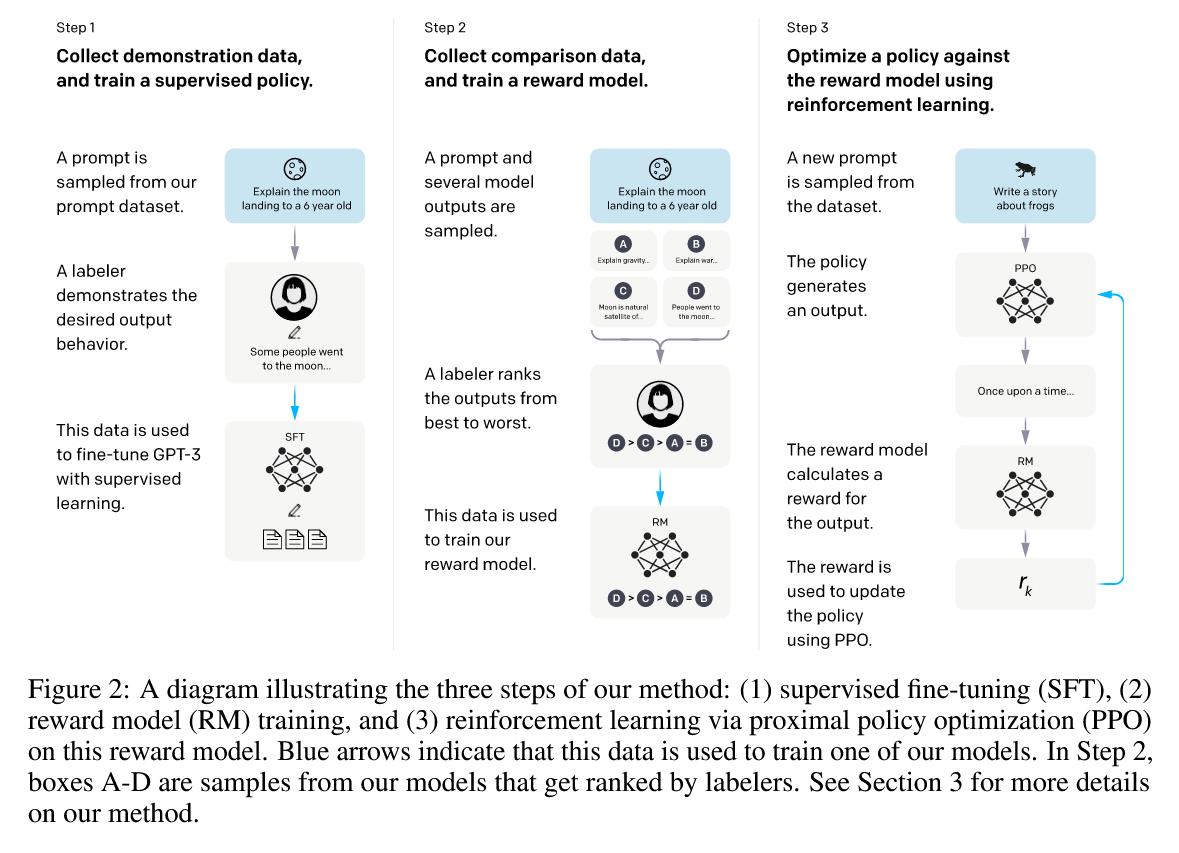
- Base Model Training
- Start with a pre-trained language model (like GPT)
- The model is initially trained on large datasets using supervised learning
- SFT: Supervised fine-tuning on high-quality data.
- Human Feedback Collection
- Human evaluators compare pairs of model outputs
- They rank which response is better based on criteria like: Helpfulness,Harmlessness, Honesty
- Reward Modeling:
- A separate neural network (reward model) is trained on human preference rankings, to predict human preferences
- This model learns to score outputs based on the collected human feedback
- It essentially learns to mimic human judgment
- Reinforcement Learning Optimization
- The original language model as policy is optimized against RM using PPO.
- The reward model provides feedback signals
- Techniques like Proximal Policy Optimization (PPO) are commonly used
- The model learns to generate responses that maximize the predicted human preference score
Benefits
- Better Alignment: Models produce outputs more consistent with human values
- Reduced Harmful Content: Helps minimize toxic, biased, or dangerous responses
- Improved Quality: Responses become more helpful and relevant
- Scalability: Once trained, the reward model can provide feedback without constant human intervention
Challenges
- Scalability of Human Feedback: Collecting sufficient high-quality human feedback is expensive and time-consuming
- Reward Hacking: Models might find ways to maximize reward scores without actually improving quality
- Bias in Human Feedback: Human evaluators may introduce their own biases
- Complexity: The multi-stage training process is computationally intensive
Reinforcement Learning from AI Feedback (RLAIF)
In Constitutional AI: Harmlessness from AI Feedback. 3, researchers introduced a paradigm that replaces human labels for harmfulness with AI-generated feedback. The approach uses a “constitution” of principles to guide self-critique and revision, enabling models to learn harmless behavior on a hybrid of human and AI preferences. This paper was the first effort to explore RLAIF.
- Key Innovation: The framework combines supervised learning (critique → revision cycles) and RL from AI Feedback (RLAIF), where a preference model (PM) is trained on AI-generated comparisons. For example, models generate pairs of responses and evaluate which aligns better with constitutional principles (e.g., “avoid harmful advice”).
- Impact: As shown in Figure 2 of the paper, Constitutional AI achieves a Pareto improvement in harmlessness and helpfulness, outperforming RLHF models that trade off these traits. The approach reduces reliance on human labeling, a critical step toward scalable supervision.
This work laid the groundwork for self-supervised RM, demonstrating that models can learn to evaluate their own behavior using explicit principles.
In RLAIF vs. RLHF: Scaling Reinforcement Learning from Human Feedback with AI Feedback 4, RLAIF achieved comparable performance to RLHF.
II. Improve Value Functioning and Eliminating Critic Model
The PPO algorithm necessitates loading four models, each of substantial size, which introduces considerable engineering complexity in the design of multi-model training, inference, and real-time parameter updates. This process demands a significant amount of GPU resources.
For instance, during RLHF training, when the Actor, Critic, Reward, and Ref Models are of identical scale, such as 70B, employing vLLM/TensorRT-llm for PPO sample generation acceleration and DeepSpeed/Megatron for training acceleration results in roughly equal computational resource consumption between inference and training stages. Consequently, the Critic model accounts for approximately one-quarter of the total computational resource usage.
In the context of LLMs, it is common for only the final token to receive a reward score from the reward model. This practice can complicate the training of a value function that accurately reflects each token’s contribution. To address this challenge, numerous studies focus on optimizing the calculation of the value function, incidentally simplifying or potentially eliminating the need for the Critic model in the process.
Group Relative Policy Optimization (GRPO)
Group Relative Policy Optimization (GRPO)5 is an efficient training algorithm proposed in the DeepSeekMath paper to enhance mathematical reasoning in language models.
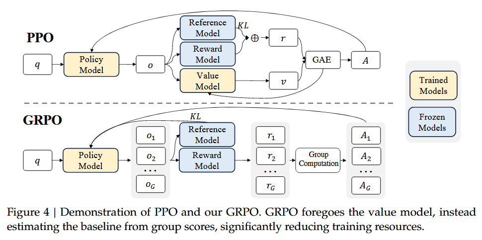
GRPO is a variant of PPO that eliminates the need for a critic model (value function), instead estimating the baseline from group-averaged rewards. This reduces memory and computational costs significantly, making it more resource-efficient.
Key Differences from PPO
- No Value Function: Unlike PPO, which uses a learned value function to compute advantages, GRPO calculates advantages using relative rewards within a group of sampled outputs for the same question.
- Group-based Baseline: For each question $q$, GRPO samples $ G $ outputs from the old policy. The baseline is the average reward of these outputs, and advantages are normalized within the group.
- Simplified Objective: GRPO optimizes the policy by maximizing a objective that uses group-relative advantages, avoiding the complexity of value function training.
How GRPO Works
Sampling: For each question $q$, sample $G$ outputs $\{o_1, o_2, \dots, o_G\}$ from the old policy $\pi_{\theta_{\text{old}}}$.
Outcome Reward Scoring and Normalization: Use a reward model to score each output, yielding $\{r_1, r_2, \dots, r_G\}$. Outcome supervision provides the normalized reward at the end of each output $o_i$ and sets the advantages $\hat{A}_{i,t}$ of all tokens in the output as the normalized reward by subtracting the group mean and dividing by the standard deviation:
$$ \hat{A}_{i,t} = \tilde{r}_i = \frac{r_i - \text{mean}(r)}{\text{std}(r)} $$Policy Update: Maximize the GRPO objective, which includes a KL divergence term to regularize against a reference model. optimizes the policy model by maximizing the following objective:
$$ \begin{aligned} \mathcal{J}_{\text{GRPO}}(\theta) &= \mathbb{E}\left[ q \sim P(Q), \{o_i\}_{i=1}^G \sim \pi_{\theta_{\text{old}}}(O|q) \right] \\\\ & \frac{1}{G} \sum_{i=1}^G \frac{1}{|o_i|} \sum_{t=1}^{|o_i|} \left\{ \min \left[ \frac{\pi_{\theta}(o_{i,t}|q, o_{i,\lt t})}{\pi_{\theta_{\text{old}}}(o_{i,t}|q, o_{i,\lt t})} \hat{A}_{i,t}, \text{clip} \left( \frac{\pi_{\theta}(o_{i,t}|q, o_{i,\lt t})}{\pi_{\theta_{\text{old}}}(o_{i,t}|q, o_{i,\lt t})}, 1 - \epsilon, 1 + \epsilon \right) \hat{A}_{i,t} \right] - \beta \mathbb{D}_{\text{KL}} \left[ \pi_{\theta} \| \pi_{\text{ref}} \right] \right\} \end{aligned} $$where $\epsilon$ and $\beta$ are hyper-parameters, and $\hat{A}_{i,t}$ is the advantage calculated based on relative rewards of the outputs inside each group only, which will be detailed in the following subsections.
- Also note that, instead of adding KL penalty in the reward, GRPO regularizes by directly adding the KL divergence between the trained policy and the reference policy to the loss, avoiding complicating the calculation of $\hat{A}_{i,t}$.
- PPO approach:
# Modify the reward with KL penalty reward_with_kl = reward - beta * kl_divergence(current_policy, ref_policy) advantage = compute_advantage(values, reward_with_kl, dones) - GRPO Approach:
# Compute advantage using original reward
advantage = compute_advantage(values, reward, dones)

# Policy loss with direct KL regularization
policy_loss = -(log_probs * advantage).mean()
kl_loss = kl_divergence(current_policy, ref_policy).mean()
total_loss = policy_loss + beta * kl_loss
- PPO approach:
- And different from the KL penalty term used in PPO, GRPO estimate the KL divergence with the following unbiased estimator6:
which is guaranteed to be positive.
- Also note that, instead of adding KL penalty in the reward, GRPO regularizes by directly adding the KL divergence between the trained policy and the reference policy to the loss, avoiding complicating the calculation of $\hat{A}_{i,t}$.
Experimental Results
- DeepSeekMath-RL (7B) using GRPO surpasses all open-source models on MATH and approaches closed-source models like GPT-4.
- Iterative GRPO (updating the reward model incrementally) further boosts performance, especially in the first iteration.
- GRPO with process supervision (step-wise rewards) outperforms outcome supervision, highlighting the value of fine-grained feedback.
RLHF with GRPO - Deepseek-R1
DeepSeek-R17 is the first public model who make use of both rule-based rewards and general RLHF via GRPO.
DeepSeek-R1-Zero: Pure RL Training
- RL Algorithm: Uses Group Relative Policy Optimization (GRPO) to optimize policies without a critic model, reducing training costs.
- Reward Modeling: Relies on rule-based rewards for accuracy (e.g., math problem correctness) and format (enforcing CoT within tags), avoiding neural reward models to prevent reward hacking.
- Self-Evolution: Through RL, the model autonomously develops complex reasoning behaviors, such as reflecting on mistakes and exploring alternative solutions, leading to significant performance gains. For example, AIME 2024 pass@1 improves from 15.6% to 71.0%, and to 86.7% with majority voting.
- Limitation:
- Suffering from readability issues, such as language mixing and unstructured outputs. And
- Lack of non-reasoning tasks such as writing and factual QA is suboptimal.
- Experiences an unstable early training process.
DeepSeek-R1: Cold-Start and Multi-Stage Refinement
DeepSeek-R1 is an attempts to address the limitations of DeepSeek-R1-Zero.
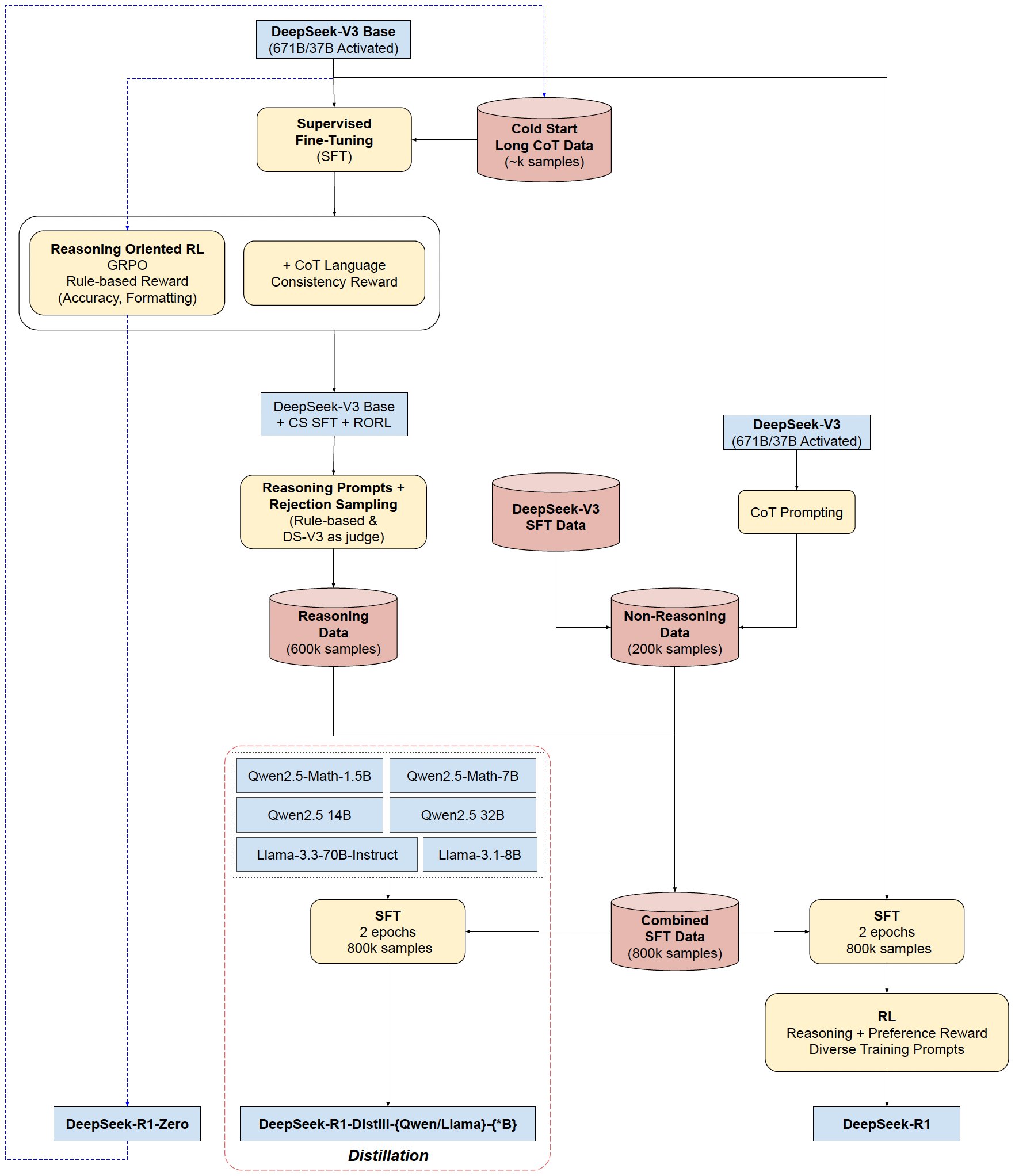
1. Cold-Start Data: Collect thousands of long CoT (chain-of-thought) examples through few-shot prompting, model-generated outputs, and human annotation. These cold-start data are used to fine-tune the DeepSeek-V3-Base to create an initial RL actor that prioritizes readable formats (e.g., summaries and structured CoT) and reducing language mixing.
2. Reasoning-Oriented RL: Apply the same large-scale reinforcement learning training process as employed in DeepSeek-R1-Zero. Incorporates language consistency rewards to mitigate mixed-language outputs, balancing performance with human readability.
3. Rejection Sampling & SFT: After RL convergence, new SFT data is collected from RL checkpoints, combining reasoning and non-reasoning tasks (e.g., writing, factual QA) to enhance general capabilities.
- For Reasoning Data Collection: Use rejection sampling on the RL checkpoint to curate ~600K reasoning samples, filtering out mixed-language and unreadable CoT. Include generative reward models (using DeepSeek-V3) for evaluation.
- For Non-Reasoning Data: Reuse SFT data from DeepSeek-V3 for tasks like writing, factual QA, and translation, collecting ~200K samples.
- Fine-Tuning: Train DeepSeek-V3-Base on the combined ~800K samples for two epochs to enhance general capabilities.
4. Scenario-Agnostic RL: A final RL stage aligns the model with human preferences for helpfulness and harmlessness, using a mix of rule-based and neural reward models.
- Reasoning Data: Use rule-based rewards for math, code, and logic tasks, as in previous stages.
- General Data: Employ reward models to capture human preferences in complex scenarios (e.g., writing, role-playing), building on DeepSeek-V3’s pipeline .
- Evaluation Focus: For helpfulness, assess the final summary; for harmlessness, evaluate the entire response (CoT and summary) to mitigate risks .
Key Advantages of Iterative RL Training
- Performance Enhancement: DeepSeek-R1 achieves comparable results to OpenAI-o1-1217 on reasoning benchmarks (e.g., 79.8% pass@1 on AIME 2024) .
- Readability and Consistency: Cold-start data and language rewards reduce language mixing and improve output structure .
- Generalization: SFT with diverse data enables competence in non-reasoning tasks like creative writing and factual QA .
Performance Benchmarks DeepSeek-R1 and distilled models excel on reasoning tasks:
- Math/Coding: AIME 2024 pass@1 of 79.8% (vs. OpenAI-o1-1217’s 79.2%), MATH-500 pass@1 of 97.3%, and Codeforces rating of 2029 (top 3.7% of human participants).
- Knowledge Tasks: MMLU score of 90.8%, GPQA Diamond of 71.5%, slightly below o1-1217 but surpassing other closed-source models.
- General Tasks: Strong performance in creative writing, summarization, and long-context understanding, with win rates of 87.6% on AlpacaEval 2.0 and 92.3% on ArenaHard.
RLOO (REINFORCE Leave One-Out)
PPO suffers from high computational costs and sensitive hyperparameter tuning. RLOO8, as a simpler RL methods, specifically REINFORCE-style optimization, can preserve or even enhance performance while reducing complexity.
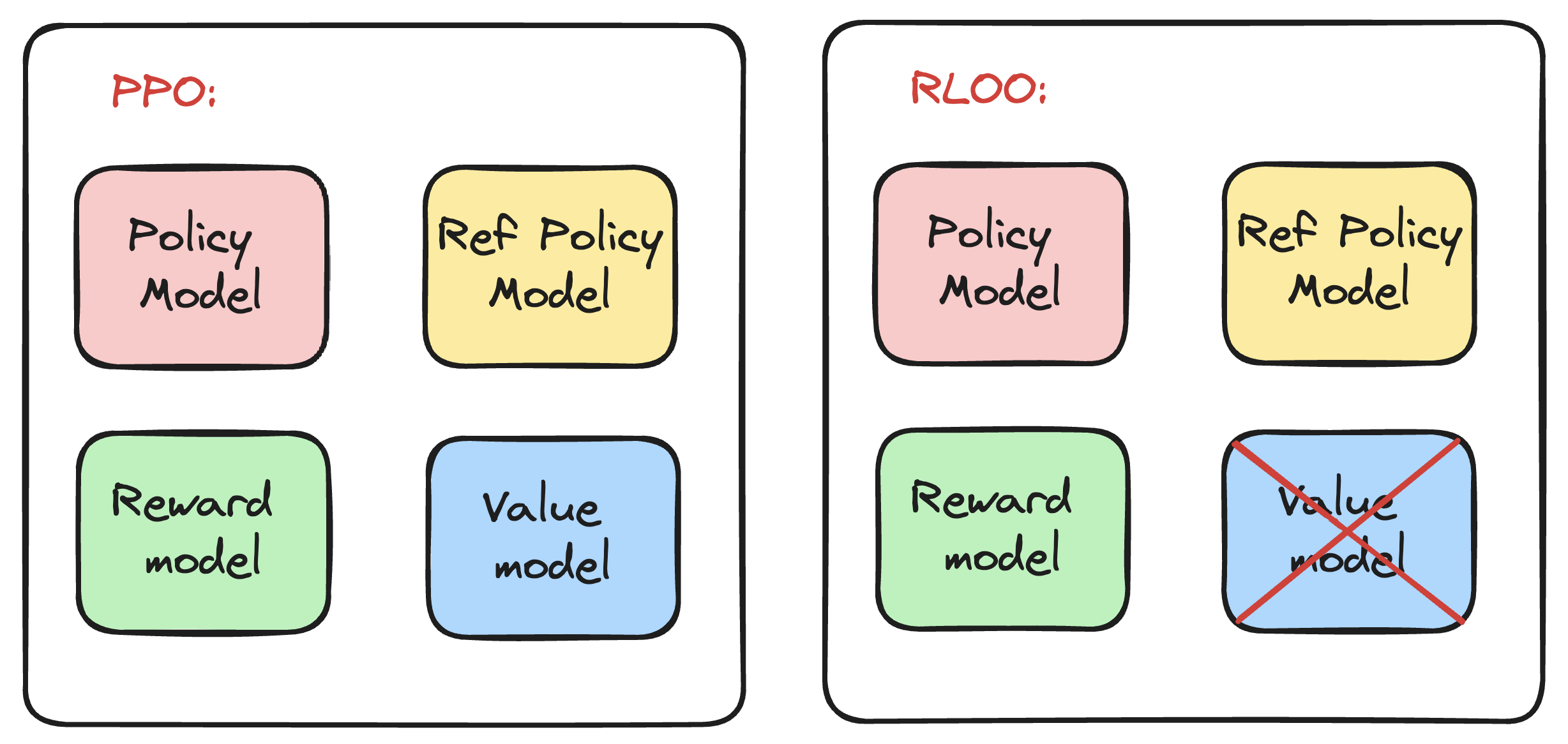
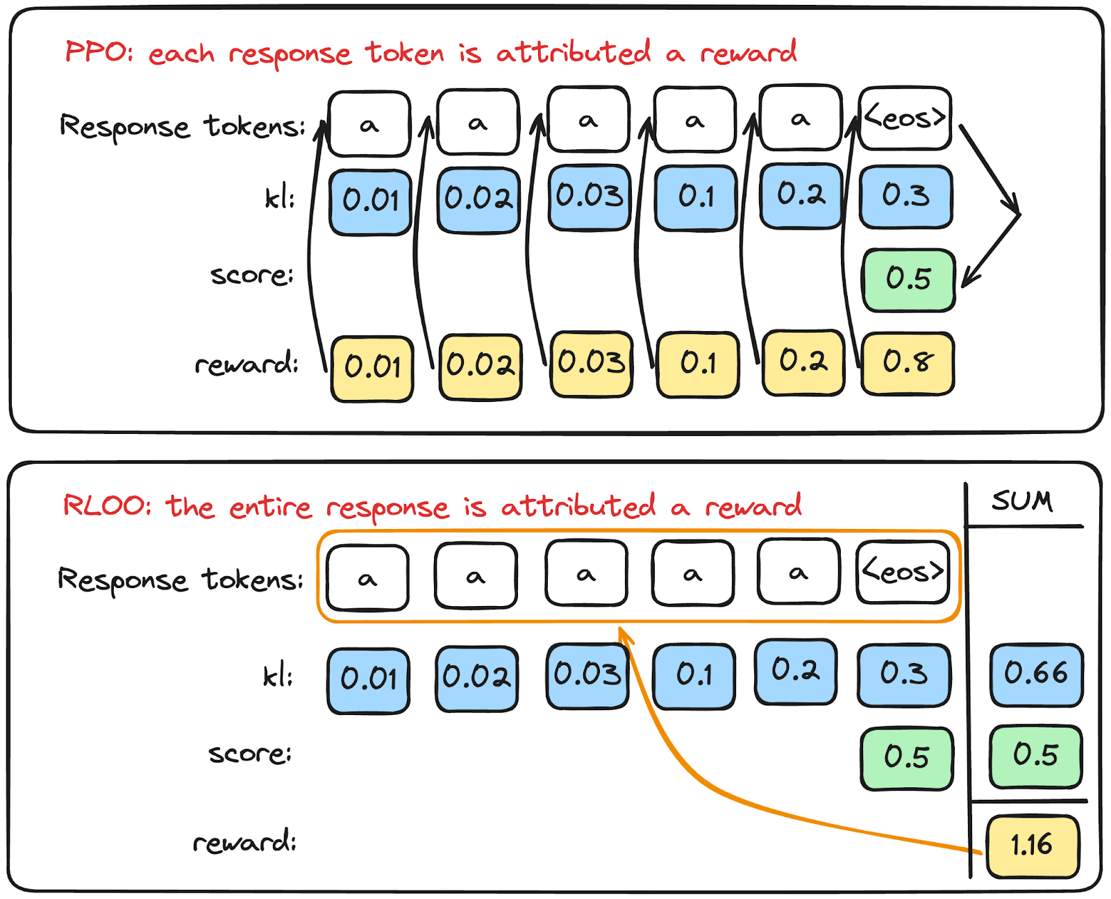 Image from https://huggingface.co/blog/putting_rl_back_in_rlhf_with_rloo 9
Key Insights:
- PPO’s Limitations in RLHF: PPO was designed for traditional RL environments with high variance and random policy initializations. In RLHF, pre-trained LLMs provide a strong policy initialization, concentrating probability mass on a small subset of tokens. This stability makes PPO’s complexity (e.g., clipping, value networks) unnecessary.
- REINFORCE for RLHF: By modeling the entire sequence generation as a single action (vs. PPO’s token-level actions), REINFORCE directly optimizes the full trajectory reward with unbiased baselines. This avoids the bias introduced by PPO’s bootstrapped value functions.
- REINFORCE Leave-One-Out (RLOO): A multi-sample extension of REINFORCE, RLOO uses online samples to create dynamic baselines, reducing variance without bias. It outperforms PPO and RL-free methods by fully leveraging all generated samples.
REINFORCE
REINFORCE loss, which applies the vanilla policy gradient to the entire sequence, using a moving average reward as a baseline.It basically multiplies the (reward - baseline) by the logprob of actions.
- Core Idea: In LLM applications, since the reward $r(x, y)$ is only available at the end of the full sequence, REINFORCE models the entire generation as a single action rather than each token. This aligns with the bandit problem formulation, where the Markov Decision Process (MDP) includes only the initial state (prompt) and the terminal state (completed sequence).
- Estimator: It uses the REINFORCE estimator to backpropagate through the discrete action space (generation) and directly optimize the KL-shaped reward objective for the entire sequence. The update rule is $$ \mathbb{E}_{x \sim \mathcal{D}, y \sim \pi_{\theta}(. | x)}\left[R(y, x) \nabla_{\theta} \log \pi_{\theta}(y | x)\right] \tag{6} $$ The intuition here is related to the likelihood principle. If an action (generation of \(y\)) leads to a high reward, we want to increase the probability of taking that action in the future, and vice versa. The REINFORCE estimator is used to update the parameters \(\theta\) of the policy \(\pi_{\theta}\). The expectation in the formula combines the reward and the policy gradient. Essentially, it tells us how to adjust the policy parameters \(\theta\) to maximize the expected reward. Mathematically, when we take the expectation of the product of the reward \(R(y, x)\) and the policy gradient \(\nabla_{\theta} \log \pi_{\theta}(y | x)\), we are computing a quantity that, when used to update \(\theta\) (using gradient ascent, for example), will tend to increase the expected reward. If \(R(y, x)\) is positive, the update will push the policy in the direction of increasing the probability of generating \(y\) given \(x\), and if \(R(y, x)\) is negative, it will push the policy away from generating \(y\) given \(x\).
- Baseline: To improve learning, one can reduce the variance of the REINFORCE estimator, while keeping it unbiased, by subtracting a baseline $b$ that has high covariance with the stochastic gradient estimate of the Eq.6: $$ \mathbb{E}_{x \sim \mathcal{D}, y \sim \pi_\theta(.|x)} \big[ (R(y, x) - b) \nabla_\theta \log \pi_\theta(y|x) \big] \tag{7} $$ The moving average of all rewards throughout training (Williams, 1992) is a strong parameter-free choice for the baseline: $$ b_{\text{MA}} = \frac{1}{S} \sum_{s} R(x^s, y^s) \tag{8} $$ Where $S$ is the number of training steps, and $(x^s, y^s)$ is the prompt-completion pair at the step $s$. This baseline is simple, computationally cheap, and parameter-free.
Noticed that REINFORCE is a special case of PPO. PPO uses importance sampling to update the policy without re-collecting data, with a clipped objective to bound policy updates: $\mathcal{L}^{\text{PPO}}(\theta) = \mathbb{E} \left[ \min \left( r_t(\theta) \cdot A_t, \text{clip}(r_t(\theta), 1-\varepsilon, 1+\varepsilon) \cdot A_t \right) \right]$, where $r_t(\theta) = \frac{\pi_\theta(a_t|s_t)}{\pi_{\theta_{\text{old}}}(a_t|s_t)}$ is the importance ratio, $A_t$ is the advantage estimate (e.g., from TD or MC), and $\varepsilon$ is the clipping parameter. To reduce PPO’s objective to REINFORCE’s with specific parameters set:
- Removing Clipping ($\varepsilon \to \infty$): When $\varepsilon$ is infinitely large, the $\text{clip}(\cdot)$ operation becomes irrelevant, and the PPO objective simplifies to: $\mathcal{L}(\theta) = \mathbb{E} \left[ r_t(\theta) \cdot A_t \right]$.
- If we further assume the old policy $\pi_{\theta_{\text{old}}}$ is the same as the current policy $\pi_\theta$ (i.e., no importance sampling, or a single update without old policy), then $r_t(\theta) = 1$, and the objective becomes: $\mathcal{L}(\theta) = \mathbb{E} \left[ A_t \right]$
- Using Monte Carlo(MC) Returns as Advantage ($A_t = G_t - b(s_t)$): If $A_t$ is defined as the MC return minus a baseline (as in REINFORCE), and the baseline $b(s_t) = 0$ (or ignored), then $A_t = G_t$. Substituting into the objective: $\mathcal{L}(\theta) = \mathbb{E} \left[ G_t \right]$, whose gradient is exactly the REINFORCE update rule without a baseline. If a baseline is included ($b(s_t) \neq 0$), it aligns with REINFORCE with a baseline, which is the standard practice to reduce variance.
— A2C Is a Special Case of PPO10
Even though the logprob is explicitly in the REINFORCE loss, it is also implicitly in the PPO loss.
REINFORCE Leave-One-Out (RLOO)
Leverages multiple online samples to further reduce variance in the REINFORCE estimator while keeping it unbiased.
For each prompt, generates k samples and uses the average reward of k-1 samples as a baseline for the remaining one, creating a variance-reduced gradient estimate.
The baseline in Eq. 8 is simple to implement and computationally cheap. However, it can be improved upon if we have access to multiple online samples, that can be used for further unbiased variance reduction:
- The rewards for each sample can serve all other samples as a baseline.
- Policy updates can be done on an average of gradient estimates for each sample, resulting in a variance-reduced multi-sample Monte-Carlo (MC) estimate.
This is the intuition behind the REINFORCE Leave-One-Out (RLOO) estimator, proposed by (Kool et al., 2019):
$$ \frac{1}{k} \sum_{i=1}^{k} \left[ R(y_{(i)}, x) - \frac{1}{k - 1} \sum_{ j \neq i} R(y_{(j)}, x) \right] \nabla \log \pi(y_{(i)} | x) \text{ for } y_{(1)}, \ldots, y_{(k)} \stackrel{i.i.d}{\sim} \pi_{\theta}(. | x) $$Where \(k\) refers to the number of online samples generated, \(\text{RLOO}_k\) considers each \( y_{(i)} \) individually and uses the remaining \( k - 1 \) samples to create an unbiased estimate of the expected return for the prompt, akin to a parameter-free value-function, but estimated at each training step.
This is a much more effective baseline (as the paper’s experiments showed) than \( b_{\text{MA}} \) since it’s created on-the-fly for each sample and at each training step, but comes at a cost of increased sampling time during training.
Noted that generating extra samples as a means of variance reduction has been proposed by concurrent work - Remax 11, but RLOO focus on the efficiency benefits of fully utilizing all samples.
Results:
- Performance: REINFORCE outperforms PPO by 3.2–20.3% in win-rate. RLOO further improves performance, surpassing DPO and RAFT across all datasets.
- Sample Efficiency: RLOO with k=2 matches or exceeds RAFT with k=4, demonstrating better use of online samples.
- Robustness: RLOO is less sensitive to KL penalty and reward noise compared to RAFT, maintaining stable performance under varying conditions.
- Alignment Tax: RLOO preserves language fluency (perplexity) and diversity better than PPO, with lower reward variance—a key factor for safety-critical applications.
ReMax
PPO introduces significant computational overhead for LLMs due to its complex architecture: it requires training a value model, leading to heavy memory usage, tedious hyperparameter tuning, and slow training. To make RLHF efficient, ReMax 11 leverages 3 properties of RLHF: fast simulation, deterministic transitions, and trajectory-level rewards. ReMax does not require training an additional value model as in PPO and is further enhanced with a new variance reduction technique.
Key limitations of PPO for RLHF:
- Value model overhead: Consumes ~46% of GPU memory for a 7B model.
- Hyperparameter complexity: Requires tuning 4+ parameters (e.g., clipping, GAE coefficient).
- Slow convergence: Training with PPO can be 4× slower than earlier RLHF steps.

Key Insights: Unique Properties of RLHF for LLMs
ReMax leverages three properties of RLHF that PPO overlooks:
- Fast simulation: Generating a complete LLM response (trajectory) is rapid (e.g., <10s for 7B models).
- Deterministic transitions: Text generation depends only on past tokens, with no stochastic environment dynamics.
- Trajectory-level rewards: Rewards are given only after the full response, not at each step.
The ReMax Algorithm
ReMax is built on the REINFORCE algorithm but introduces a variance reduction technique:
- Greedy baseline: For each prompt, compute the reward of a greedy (deterministic) response and use it to normalize the gradient, reducing variance.
- For a prompt, sample a stochastic response and a greedy response.
- Compute the reward difference between the two responses.
- No value model: Directly optimizes the policy to maximize the log-likelihood of high-reward responses, weighted by the reward difference.
Pseudo-code Core Steps:
for prompt in dataset:
    seq = lm.sample(prompt, greedy=False)         # Stochastic response
    seq_max = lm.sample(prompt, greedy=True)      # Greedy response
    rew = rm(prompt, seq) - rm(prompt, seq_max)   # Reward difference
    logp = lm.inference(prompt, seq)              # Log-likelihood
    loss = - (logp.sum() * rew).mean()            # Loss for optimization
    lm.minimize(loss)
REINFORCE++
RLOO and GRPO increase inference costs to trade for eliminating the critic model. The blog 12 argues that eliminating the critic model may inadvertently lower training efficiency due to increased inference costs:
- When all models (Actor, Critic, Reward, Reference) are similar in scale (e.g., 70B parameters), inference and training consume roughly equal computational resources (1:1 ratio). Eliminating the critic model may actually reduce training efficiency due to increased inference costs
- System complexity remains largely unchanged since multiple models still need to operate together
- Performance Analysis:
- REINFORCE-based methods (e.g., RLOO, ReMax, GRPO) eliminate the critic but struggle with accurate advantage estimation, often overfitting to simple prompts and being vulnerable to reward hacking. These methods estimate advantages per prompt, leading to instability and poor generalization.
- GRPO and RLOO don’t provide significant theoretical improvements over PPO
- The claimed advantages (like “10x” efficiency gains) are often exaggerated
- PPO can address critic model issues by initializing critics with actor weights
- Alternative solution: Pre-train the critic model by freezing actor weights during PPO training
- Technical Issues with GRPO:
- Numerical instability: Small differences in sampled rewards can be amplified during normalization
- Example: rewards of 1.001 vs 1.00 become -0.7070 vs 0.7072 after normalization
- Convergence problems: When all sampled rewards are equal, GRPO provides zero learning signal
- Under Process Reward Model (PRM) settings, GRPO essentially becomes REINFORCE with mean baseline
- Bottom Line:: Both GRPO and RLOO are most beneficial when critic/reward models are significantly larger than actors, but even then, PPO remains a viable alternative with proper initialization strategies. The computational and complexity advantages are often overstated.
REINFORCE++ 13 is a critic-free RLHF algorithm that uses the global batch mean reward as a baseline instead of prompt-specific baselines, preventing overfitting and improving robustness.
 The overall algorithm flow of REINFORCE++: Sample one response per prompt, compute rewards, normalize advantages, and update the policy using a clipped objective (similar to PPO but without the critic).
Advantages Normalization: Normalizes advantages across the entire batch to stabilize training and enhance out-of-distribution (OOD) generalization. REINFORCE++ replaces prompt-specific baselines with the mean reward of a global batch, reducing overfitting to individual prompts. The Advantage is calculated as:
$$ A_{q, o_t} = r(o_{1:t}, q) - \beta \cdot \sum_{i=t}^T KL(i), \quad \text{with } KL(t) = \log\left(\frac{\pi_{\theta_{\text{old}}}^{RL}(o_t | q, o_{\lt t})}{\pi^{\text{SFT}}(o_t | q, o_{\lt t})}\right) $$The token-level KL penalty avoids the need for a critic network while achieving comparable stability. The gradient of the token-level KL penalty has been theoretically proven to be unbiased concerning the $k_3$ loss of GRPO in RLHF.
The advantage is normalized globally:
$$ A_{q, o_t}^{\text{norm}} = \frac{A_{q, o_t} - \text{mean}(A_{q, o_t})}{\text{std}(A_{q, o_t})} $$Experimental Results:
- Bradley-Terry Reward Model: REINFORCE++ matches or exceeds performance of GRPO, RLOO, and ReMax on OOD benchmarks (e.g., GSM8K, MATH, code generation), with higher per-token efficiency.
- Long CoT Tasks:
- Small-Scale Datasets: GRPO overfits to training prompts (e.g., AIME-24), achieving near-perfect scores but failing on OOD test sets (AIME-25), while REINFORCE++ shows stable generalization.
- Logical Reasoning (Knights and Knaves): REINFORCE++ outperforms GRPO in complex and OOD scenarios (e.g., 8-character puzzles), with higher Pass@1 scores (36 vs. 20) and longer, more reasoned responses.
- Mathematical Reasoning: From scratch or fine-tuned models, REINFORCE++ demonstrates better OOD generalization on MATH and AIME datasets.
DAPO (Decoupled Clip and Dynamic Sampling Policy Optimization)
DAPO 14 decouples policy clipping and dynamic sampling to enhance training efficiency, reducing variance in gradient estimates.
DAPO addresses critical challenges in RL training—such as entropy collapse, reward noise, and instability—with four key techniques.
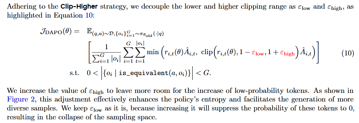
- Clip-Higher: Decouples lower $\varepsilon_{low}$ and higher $\varepsilon_{high}$ clipping ranges in policy optimization to prevent entropy collapse. By increasing $\varepsilon_{high}$, low-probability “exploration” tokens gain more room for probability increases, enhancing diversity.
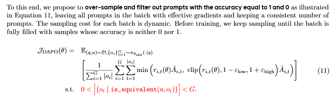
- Dynamic Sampling: Over-samples and filters out prompts with all-correct or all-wrong outputs to maintain effective gradient signals. This mitigates gradient-decreasing issues from zero-advantage batches, improving training efficiency.
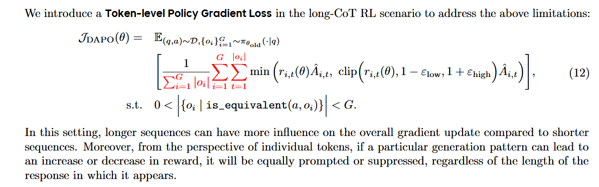
- Token-Level Policy Gradient Loss: Shifts from sample-level to token-level loss calculation, balancing the influence of long and short responses. This prevents low-quality, overly long generations and stabilizes training.
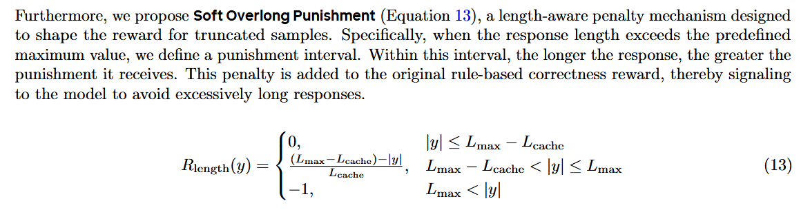
- Overlong Reward Shaping: Introduces soft punishment for truncated responses to reduce reward noise. Instead of harsh penalties, it uses a length-aware function to guide models toward optimal response lengths.
Dataset and Implementation
The DAPO-Math-17K dataset transforms math problems into integer answers for reliable rule-based reward signals. The system is built on the verl framework, with training details including AdamW optimization, group reward normalization, and dynamic sampling hyperparameters.
Experiments and Results
- AIME 2024 Performance: DAPO achieves 50 points on AIME with Qwen2.5-32B, outperforming DeepSeek-R1-Zero-Qwen-32B (47 points) with half the training steps (Figure 1).
- Ablation Study: Each technique contributes significantly: Overlong Filtering (+6), Clip-Higher (+2), Soft Overlong Punishment (+3), Token-Level Loss (+1), and Dynamic Sampling (+8) (Table 1).
- Training Dynamics: Metrics like response length, reward, and entropy show stable improvement, with Clip-Higher specifically combating entropy collapse (Figure 7).
Dr. GRPO
Dr. GRPO 15 claims that:
- DeepSeek-V3-Base already exhibit “Aha moment”, while Qwen2.5 base models demonstrate strong reasoning capabilities even without prompt templates, suggesting potential pretraining biases.
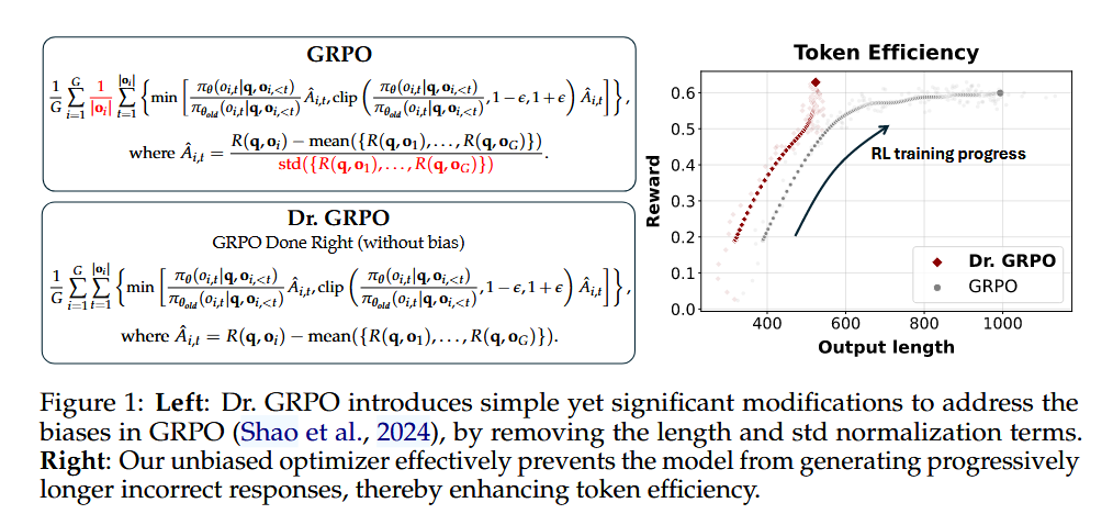
- There is an optimization bias in Group Relative Policy Optimization (GRPO), which artificially increases response length (especially for incorrect outputs) during training.
- Dr. GRPO is an unbiased optimization method that improves token efficiency while maintaining reasoning performance.
Key Insights on Base Models
Template Impact on Question-Answering Ability
- Base models like Llama and DeepSeek require prompt templates (e.g., R1 template) to elicit question-answering behavior, while Qwen2.5 models excel without templates. This suggests Qwen2.5 might be pretrained on question-answer pairs, acting like supervised fine-tuned (SFT) models even in their base form.
- For example, Qwen2.5-Math-7B achieves 69.0% accuracy on MATH500 without templates, outperforming traditional prompting methods.
Preexisting “Aha Moment” in Base Models
- The “Aha moment” (self-reflection behaviors) often attributed to RL emergence is already present in base models like DeepSeek-V3-Base. Experiments show these models generate self-reflection keywords (e.g., “Aha,” “wait”) in responses to math problems without RL tuning.
Analysis of Reinforcement Learning
Biases in GRPO
- GRPO introduces two key biases:
- Response-length bias: Dividing by response length ($|o_i|$) penalizes short correct responses and favors longer incorrect ones.
- Question-difficulty bias: Normalizing by reward standard deviation prioritizes easy/hard questions, skewing optimization.
- These biases lead to unnecessarily long incorrect responses, as observed in training dynamics.
- GRPO introduces two key biases:
Dr. GRPO: Unbiased Optimization
- The authors propose Dr. GRPO, which removes $|o_i|$ and standard deviation normalization from GRPO. This fixes the biases, improving token efficiency while maintaining reasoning performance.
- Experiments show Dr. GRPO reduces the length of incorrect responses and matches the accuracy of GRPO with fewer tokens.
The implementation from trl
class GRPOConfig(TrainingArguments):
    """
    scale_rewards (`bool`, *optional*, defaults to `True`):
            Whether to scale the rewards by dividing them by their standard deviation. If `True` (default), the rewards
            are normalized by the standard deviation, ensuring they have unit variance. If `False`, no scaling is
            applied. The [Dr. GRPO](https://github.com/sail-sg/understand-r1-zero/blob/main/understand-r1-zero.pdf)
            paper recommends not scaling the rewards, as scaling by the standard deviation introduces a question-level
            difficulty bias.
    """
    ...


class GRPOTrainer(Trainer):

    def _generate_and_score_completions(
        self, inputs: dict[str, Union[torch.Tensor, Any]]
    ) -> dict[str, Union[torch.Tensor, Any]]:
        ...

        # Gather the reward per function: this part is crucial, because the rewards are normalized per group and the
        # completions may be distributed across processes
        rewards_per_func = gather(rewards_per_func)

        # Apply weights to each reward function's output and sum
        rewards = (rewards_per_func * self.reward_weights.to(device).unsqueeze(0)).nansum(dim=1)

        # Compute grouped-wise rewards
        mean_grouped_rewards = rewards.view(-1, self.num_generations).mean(dim=1)
        std_grouped_rewards = rewards.view(-1, self.num_generations).std(dim=1)

        # Normalize the rewards to compute the advantages
        mean_grouped_rewards = mean_grouped_rewards.repeat_interleave(self.num_generations, dim=0)
        std_grouped_rewards = std_grouped_rewards.repeat_interleave(self.num_generations, dim=0)
        advantages = rewards - mean_grouped_rewards
        if self.args.scale_rewards:  # the original GRPO
            advantages = advantages / (std_grouped_rewards + 1e-4)

        ...
Group-in-Group Policy Optimization (GiGPO) for LLM Agent Training
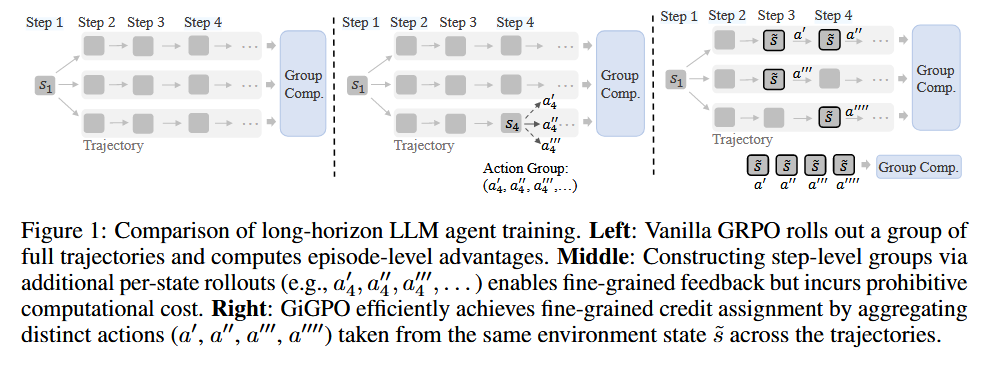
GiGPO16 is designed to enhance long-horizon training for LLM agents. Unlike existing group-based RL methods (e.g., GRPO) that struggle with fine-grained credit assignment in multi-step tasks, GiGPO achieves hierarchical advantage estimation while retaining key benefits: being critic-free, memory-efficient, and computationally lightweight.
Key Limitations of Existing Group-based RL:
- Traditional group-based RL (e.g., GRPO, RLOO) works well for single-turn tasks (e.g., math reasoning) where rewards are immediate but fails in long-horizon scenarios.
- In multi-step environments (e.g., embodied navigation, web shopping), rewards are sparse/delayed, making it hard to assign credit to individual steps.
- Naive extensions of group-based RL collapse step-level distinctions, reducing effectiveness in agent training.
GiGPO’s hierarchical “group-in-group” design:
Episode-Level Grouping:
- Objective: Capture holistic trajectory quality.
- Method: Samples a group of complete trajectories under identical initial conditions and task descriptions. Computes macro relative advantages using total episode returns, normalized by the group’s mean and a scaling factor (either standard deviation or 1 for stability). $$ A^E(\tau_i) = \frac{R(\tau_i) - \text{mean}(\{R(\tau_j)\})}{F_{\text{norm}}(\{R(\tau_j)\})} $$ where \( R(\tau_i) \) is the total reward of trajectory \( \tau_i \)
Step-Level Grouping:
- Objective: Evaluate local step effectiveness.
- Method: Identifies anchor states (repeated environment states across trajectories) to form step-level groups. Computes micro relative advantages using discounted future rewards for actions taken at these shared states. $$ A^S(a_t^{(i)}) = \frac{R_t^{(i)} - \text{mean}(\{R_t^{(j)}\})}{F_{\text{norm}}(\{R_t^{(j)}\})} $$ where \( R_t^{(i)} \) is the discounted return from step \( t \) in trajectory \( i \)
GiGPO Combined Advantage Signal: The final advantage for each action merges both levels,
$$ A(a_t^{(i)}) = A^E(\tau_i) + \omega \cdot A^S(a_t^{(i)}) $$where \( \omega \) balances the two signals.
GiGPO was evaluated on two challenging benchmarks using Qwen2.5-1.5B-Instruct and Qwen2.5-7B-Instruct:
| Benchmark | Improvement Over GRPO | Key Findings |
|---|---|---|
| ALFWorld | 12-13% higher success | Superior performance in embodied household task planning. |
| WebShop | >9% higher success | Better at goal-driven web navigation and shopping tasks. |
- Efficiency: GiGPO matches GRPO’s GPU memory usage and rollout costs, with <0.002% additional computation time.
- Ablation Studies: Removing either episode-level or step-level advantages significantly degrades performance, confirming the value of hierarchy.
Group Sequence Policy Optimization (GSPO)
The authors identify that GRPO’s objective is mathematically ill-posed due to a misapplication of importance sampling. Importance sampling estimates expectation under target distribution by re-weighting samples from behavior distribution. The sampling needs multiple samples (N ≫ 1) for correction to work. However, GRPO applies token-level importance sampling to sequence-level rewards:
- Token-level importance sampling: GRPO computes importance weights for each individual token $$w_{i,t}(\theta) = \frac{\pi_\theta(y_{i,t}|x,y_{i,\lt t})}{\pi_{\theta_{\text{old}}}(y_{i,t}|x,y_{i,\lt t})}$$
- Sequence-level rewards: The actual reward/advantage is calculated for the entire generated response
This misalignment introduces high-variance noise into training gradients that leads to high-variance noise that accumulates over long sequences, and catastrophic, irreversible model collapse
GSPO17 defines the importance ratio based on sequence likelihood (not token likelihood):
$$s_i(\theta) = \left(\frac{\pi_\theta(y_i|x)}{\pi_{\theta_{\text{old}}}(y_i|x)}\right)^{\frac{1}{|y_i|}} = \exp\left(\frac{1}{|y_i|}\sum_{t=1}^{|y_i|}\log\frac{\pi_\theta(y_{i,t}|x,y_{i,\lt t})}{\pi_{\theta_{\text{old}}}(y_{i,t}|x,y_{i,\lt t})}\right)$$which uses geometric mean of token-level ratios (via log-space averaging), with length normalization to reduce variance.
The objective function is then defined as:
$$\mathcal{J}_{\text{GSPO}}(\theta) = \mathbb{E}_{x\sim\mathcal{D},\{y_i\}_{i=1}^G\sim\pi_{\theta_{\text{old}}}(\cdot|x)}\left[\frac{1}{G}\sum_{i=1}^G \min\left(s_i(\theta)\hat{A}_i, \text{clip}(s_i(\theta), 1-\varepsilon, 1+\varepsilon)\hat{A}_i\right)\right]$$with clipping applies to entire responses, not individual tokens. Where advantages are computed group-wise (same as GRPO):
$$\hat{A}_i = \frac{r(x,y_i) - \text{mean}(\{r(x,y_i)\}_{i=1}^G)}{\text{std}(\{r(x,y_i)\}_{i=1}^G)}$$Why GSPO Works Better: Gradient Analysis
In GRPO’s gradient, tokens are unequally weighted by their individual importance ratios:
$$\nabla_\theta \mathcal{J}_{\text{GRPO}}(\theta) = \mathbb{E}\left[\frac{1}{G}\sum_{i=1}^G \hat{A}_i \cdot \frac{1}{|y_i|}\sum_{t=1}^{|y_i|} \underbrace{\frac{\pi_\theta(y_{i,t}|x,y_{i,\lt t})}{\pi_{\theta_{\text{old}}}(y_{i,t}|x,y_{i,\lt t})}}_{\text{unequal, varying weights}} \nabla_\theta \log\pi_\theta(y_{i,t}|x,y_{i,\lt t})\right]$$Weights vary wildly: $(0, 1+\varepsilon]$ for positive advantage, $[1-\varepsilon, +\infty)$ for negative advantage.
In GSPO’s gradient, all tokens in a sequence are equally weighted:
$$\nabla_\theta \mathcal{J}_{\text{GSPO}}(\theta) = \mathbb{E}\left[\frac{1}{G}\sum_{i=1}^G \left(\frac{\pi_\theta(y_i|x)}{\pi_{\theta_{\text{old}}}(y_i|x)}\right)^{\frac{1}{|y_i|}} \hat{A}_i \cdot \frac{1}{|y_i|}\sum_{t=1}^{|y_i|} \nabla_\theta \log\pi_\theta(y_{i,t}|x,y_{i,\lt t})\right]$$The sequence-level ratio $s_i(\theta)$ is constant across all tokens in the response, eliminating the instability source.
By aligning all operations at the sequence level, GSPO eliminates the variance mismatch that plagues GRPO.
| Aspect | GRPO | GSPO |
|---|---|---|
| Importance Ratio | Token-level | Sequence-level (based on total sequence likelihood) |
| Clipping | Per-token | Per-sequence |
| Reward/Advantage | Sequence-level | Sequence-level |
| Optimization | Token-level | Sequence-level |
Benefits for the Mixture-of-Experts(MoE) Challenge
In MoE models, expert activation volatility causes problems: After each gradient update, ~10% of activated experts change for the same input. This makes token-level importance ratios fluctuate drastically. Previously, we use Routing Replay to stabilize GRPO training. Specifically, we store the routing decisions (cache which experts were activated under old policy) for each training sample and replay the same routing when computing new policy probabilities, to ensure consistent importance ratios. However, this is a workaround that adds complexity and overhead.
GSPO eliminates the need for Routing Replay entirely as it only cares about sequence likelihood $\pi_\theta(y_i|x)$, which is not sensitive to which specific experts activate for each token.
Infrastructure Benefits
Token-level likelihoods must recompute the likelihood with training engine (Megatron) due to precision discrepancies with inference engines.
While sequence-level likelihoods are more tolerant of precision discrepancies than token-level likelihoods. Hence we can use inference engine likelihoods directly (SGLang, vLLM), which enables partial rollout, multi-turn RL, training-inference disaggregation.
Training Stability & Efficiency
The experiments use Qwen3-30B-A3B-Base (a 30B parameter MoE model with 3B active parameters). GSPO shows continuous, stable improvement with more compute, and achieves better performance with same training compute.
The Clipping Paradox
Counter-intuitively, GSPO clips ~100× more tokens (15% vs 0.13%) yet trains more efficiently.
GSPO-token: GSPO with token-level advantages
For scenarios needing finer-grained control (e.g., multi-turn RL), the authors propose GSPO-token:
$$s_{i,t}(\theta) = \underbrace{\text{sg}[s_i(\theta)]}_{\text{sequence ratio (no grad)}} \cdot \frac{\pi_\theta(y_{i,t}|x,y_{i,\lt t})}{\text{sg}[\pi_\theta(y_{i,t}|x,y_{i,\lt t})]}$$which is numerically equals $s_i(\theta)$ (as $\frac{\pi_\theta}{\text{sg}[\pi_\theta]} = 1$). The sg[·] denotes only taking the numerical value but stopping the gradient, corresponding to the detach operation in PyTorch. During backprop, gradient flows through $\pi_\theta(y_{i,t})$ normally, and $s_i(\theta)$ acts as a constant multiplier (like a learning rate adjustment).
The key difference to GRPO is what gets clipped: The clipping unit in GRPO is individual tokens, while in GSPO-token, the clipping unit is the entire sequence (via $s_i(\theta) = \left(\frac{\pi_\theta(y_i\|x)}{\pi_{\theta_{\text{old}}}(y_i\|x)}\right)^{\frac{1}{\|y_i\|}}$).
GRPO (Token-Level Clipping):
$$\mathcal{J}_{\text{GRPO}}(\theta) = \mathbb{E}\left[\frac{1}{G}\sum_{i=1}^G \frac{1}{|y_i|}\sum_{t=1}^{|y_i|} \min\left(w_{i,t}(\theta)\hat{A}_i, \text{clip}(w_{i,t}(\theta), 1-\epsilon, 1+\epsilon)\hat{A}_i\right)\right]$$Where:
$$w_{i,t}(\theta) = \frac{\pi_\theta(y_{i,t}|x,y_{i,\lt t})}{\pi_{\theta_{\text{old}}}(y_{i,t}|x,y_{i,\lt t})}$$Each token is clipped individually, leads to high variance, noisy decisions. Gradient (Token-Weighted Chaos):
$$\nabla_\theta \mathcal{J}_{\text{GRPO}} = \mathbb{E}\left[\frac{1}{G}\sum_{i=1}^G \hat{A}_i \cdot \frac{1}{|y_i|}\sum_{t=1}^{|y_i|} \underbrace{w_{i,t}(\theta)}_{\text{token weight}} \nabla_\theta \log\pi_\theta(y_{i,t}|x,y_{i,\lt t})\right]$$Each token weighted by its own volatile ratio, leads to gradients explode/vanish unpredictably.
GSPO-token (Sequence-Level Clipping, Token-Level Advantages):
$$\mathcal{J}_{\text{GSPO-token}}(\theta) = \mathbb{E}\left[\frac{1}{G}\sum_{i=1}^G \frac{1}{|y_i|}\sum_{t=1}^{|y_i|} \min\left(s_{i,t}(\theta)\hat{A}_{i,t}, \text{clip}(s_{i,t}(\theta), 1-\epsilon, 1+\epsilon)\hat{A}_{i,t}\right)\right]$$Where:
$$s_{i,t}(\theta) = \underbrace{\text{sg}\left[s_i(\theta)\right]}_{\text{sequence ratio, no grad}} \cdot \frac{\pi_\theta(y_{i,t}|x,y_{i,\lt t})}{\text{sg}\left[\pi_\theta(y_{i,t}|x,y_{i,\lt t})\right]}$$the clipping is based on the sequence ratio $s_i(\theta)$, not the token ratio. GSPO-token Gradient (Sequence-Weighted Stability):
$$\nabla_\theta \mathcal{J}_{\text{GSPO-token}} = \mathbb{E}\left[\frac{1}{G}\sum_{i=1}^G \underbrace{s_i(\theta)}_{\text{sequence weight}} \cdot \frac{1}{|y_i|}\sum_{t=1}^{|y_i|} \hat{A}_{i,t} \nabla_\theta \log\pi_\theta(y_{i,t}|x,y_{i,\lt t})\right]$$All tokens weighted by same stable sequence ratio.
III. Optimization without Reward Model
Direct Preference Optimization (DPO)
DPO18 is a RL-free training method for LLMs that directly optimizes for human preferences without requiring a separate reward model. DPO eliminates the need for a reward model by directly optimizing a policy using pairwise preference data. It minimizes the KL divergence between the policy and a reference model while maximizing the Bradley-Terry loss.
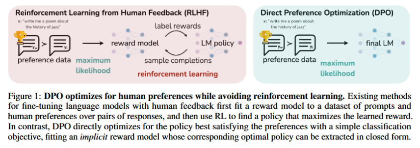
DPO derives a closed-form solution that directly optimizes the policy using preference data. The key insight is that the optimal policy under the RLHF objective can be expressed analytically in terms of the reward function and reference policy.
The DPO objective is based on the Bradley-Terry preference model, the optimal RLHF policy $π^∗$ under the Bradley-Terry model satisfies the preference model::
$$P(y_w \succ y_l | x) = \frac{1}{1 + \exp(\beta \log \frac{\pi_\theta(y_l|x)}{\pi_{ref}(y_l|x)} - \beta \log \frac{\pi_\theta(y_w|x)}{\pi_{ref}(y_w|x)})}$$Where:
- $y_w$ is the preferred (winning) response
- $y_l$ is the less preferred (losing) response
- $x$ is the input prompt
- $\pi_\theta$ is the policy being optimized
- $\pi_{ref}$ is the reference policy
- $\beta$ is a temperature parameter
For a static dataset of comparisons $\mathcal{D} = \left\{ x^{(i)}, y_w^{(i)}, y_l^{(i)} \right\}_{i=1}^N$, the reward modeling approach works by defining:
$$ \mathcal{L}_R(r_\phi, \mathcal{D}) = -\mathbb{E}_{(x, y_w, y_l) \sim \mathcal{D}} \left[ \log \sigma \left( r_\phi(x, y_w) - r_\phi(x, y_l) \right) \right] $$Analogous to reward modeling approach, DPO’s policy objective becomes:
$$ \mathcal{L}_{\text{DPO}}(\pi_\theta; \pi_{\text{ref}}) = -\mathbb{E}_{(x, y_w, y_l) \sim \mathcal{D}} \left[ \log \sigma \left( \beta \log \frac{\pi_\theta(y_w \mid x)}{\pi_{\text{ref}}(y_w \mid x)} - \beta \log \frac{\pi_\theta(y_l \mid x)}{\pi_{\text{ref}}(y_l \mid x)} \right) \right] $$The gradient with respect to the parameters $\theta$ can be written as:
$$ \nabla_\theta \mathcal{L}_{\text{DPO}}(\pi_\theta; \pi_{\text{ref}}) = - \beta \mathbb{E}_{(x,y_w,y_l) \sim \mathcal{D}} \bigg[ \underbrace{\sigma\bigl(\hat{r}_\theta(x, y_l) - \hat{r}_\theta(x, y_w)\bigr)}_{\text{higher weight when reward estimate is wrong}} \, \bigg[ \underbrace{\nabla_\theta \log \pi(y_w \mid x)}_{\text{increase likelihood of } y_w} - \underbrace{\nabla_\theta \log \pi(y_l \mid x)}_{\text{decrease likelihood of } y_l} \bigg] \bigg] $$where $\hat{r}_\theta(x, y) = \beta \log \frac{\pi_\theta(y \mid x)}{\pi_{\text{ref}}(y \mid x)}$ is the reward implicitly defined by the language model $\pi_\theta$ and reference model $\pi_{\text{ref}}$.
A mechanistic understanding of DPO
- The gradient of the loss function $\mathcal{L}_{\text{DPO}}$ increases the likelihood of the preferred completions $y_w$ and decreases the likelihood of dispreferred completions $y_l$.
- The examples are weighed by how much higher the implicit reward model $\hat{r}_\theta$ rates the dispreferred completions, scaled by $\beta$, i.e, how incorrectly the implicit reward model orders the completions, accounting for the strength of the KL constraint.
- The papers’s experiments suggest the importance of this weighting, as a naïve version of this method without the weighting coefficient can cause the language model to degenerate.
DPO’s Training Process
- Data Collection: Gather preference pairs $(x, y_w, y_l)$ where $y_w$ is preferred over $y_l$ for prompt $x$
- Direct Optimization: Minimize the DPO loss $\mathcal{L}_{\text{DPO}}$
- Regularization: The KL divergence constraint from RLHF is implicitly maintained through the reference policy terms
Advantages of DPO
- Simplicity
- Eliminates the need for reward model training
- Reduces the training pipeline from 3 stages to 2 stages
- Avoids the complexities of reinforcement learning
- Stability
- More stable training compared to PPO-based RLHF
- No issues with reward model overoptimization
- Direct gradient-based optimization
- Efficiency
- Requires less computational resources
- Faster convergence
- Easier hyperparameter tuning
Practical Implementation
# Simplified DPO loss computation
def dpo_loss(policy_chosen_logps, policy_rejected_logps,
             reference_chosen_logps, reference_rejected_logps, beta=0.1):
    policy_logratios = policy_chosen_logps - policy_rejected_logps
    reference_logratios = reference_chosen_logps - reference_rejected_logps

    logits = beta * (policy_logratios - reference_logratios)
    loss = -torch.nn.functional.logsigmoid(logits).mean()

    return loss
Limitations and Considerations
- Data Quality: Heavily dependent on high-quality preference data
- Distribution Shift: May struggle with significant shifts from reference policy
- Preference Complexity: Works best with clear preference distinctions
- Hyperparameter Sensitivity: The β parameter requires careful tuning
Comparison with RLHF
| Aspect | RLHF | DPO |
|---|---|---|
| Complexity | High (3 stages) | Medium (2 stages) |
| Stability | Can be unstable | More stable |
| Computational Cost | High | Lower |
| Flexibility | High | Moderate |
Online DPO - Direct Language Model Alignment from Online AI Feedback
Direct Alignment from Preferences (DAP) methods like DPO have emerged as efficient alternatives to RLHF, but they rely on pre-collected offline preference data. This leads to two key issues:
- Offline Feedback: Preferences are static and not updated during training.
- Off-Policy Learning: Responses in the dataset are generated by a different model, causing distribution shift as the target model evolves.
The proposed Online AI Feedback (OAIF) framework19 makes Online DAP methods online and on-policy by:
- Sampling two responses from the current model for each prompt.
- Using an LLM annotator (e.g., PaLM 2) to provide real-time preference feedback by choosing the better response.
- Updating the model using standard DAP losses (DPO, IPO, SLiC) with this online feedback.
Key advantages:
- Avoids distribution shift by using on-policy generations.
- Eliminates the need for a separate Reward Model (RM), unlike RLHF.
- Enables controllable feedback via prompt engineering for the LLM annotator.
Experiments and Results
Effectiveness vs. Offline DAP:
- Online DAP methods (DPO, IPO, SLiC) achieved an average 66% win rate over their offline counterparts in human evaluations.
- Online DPO outperformed SFT baselines, RLHF, and RLAIF 58% of the time on the TL;DR task.
Generalization to Other DAP Methods:
- OAIF improved all three DAP methods, with online SLiC showing a 71.43% win rate over offline SLiC in TL;DR.
Comparison with RLHF/RLAIF:
- Online DPO was preferred 58% of the time in 4-way comparisons (vs. offline DPO, RLAIF, RLHF).
- RLHF relies on static RMs, which struggle as the model evolves, while OAIF’s LLM annotator adapts dynamically.
Controllability via Prompts:
- Instructing the LLM annotator to prefer shorter responses reduced average token length from ~120 to ~40, while maintaining quality above SFT baselines.
Impact of Annotator Size:
- Larger annotators (e.g., PaLM 2-L) improved performance, but even smaller annotators (PaLM 2-XS) outperformed RLHF in some cases.
OAIF addresses the offline and off-policy limitations of DAP methods, achieving better alignment with reduced human annotation. The approach paves the way for scalable LLM alignment using AI feedback, with potential for real-time user adaptation and qualitative objective control.
| Method | No RM Needed | On-Policy | Online Feedback |
|---|---|---|---|
| Offline DAP | ✓ | ✗ | ✗ |
| RLHF/RLAIF | ✗ | ✓ | ✓ |
| OAIF (Proposed) | ✓ | ✓ | ✓ |
TDPO: Token-level Direct Preference Optimization
DPO optimize models at the sentence level, evaluating full responses. However, LLMs generate text token-by-token in an auto-regressive manner, which creates a mismatch between evaluation and generation processes. DPO uses KL divergence to constrain models to a reference LLM but struggles with divergence efficiency: the KL divergence of dispreferred responses grows too quickly, limiting diversity. This motivates the need for a more granular, token-level optimization approach.
TDPO20 optimizes token-level preferences to improve sequence generation quality, addressing limitations of instance-level DPO in long-chain reasoning.

TDPO models text generation as an MDP, where:
- State \( s_t = [x, y^{\lt t}] \) (prompt + partial response)
- Action \( a_t = y^t \) (next token)
- Reward \( R_t := R(s_t, a_t) = R\bigl([x, y^{\lt t}], y^t\bigr). \) (token-wise reward)
The objective function combines the advantage function of a reference model with forward KL divergence:
\[ \max_{\pi_\theta} \mathbb{E}\left[ A_{\pi_{ref}}(s_t, z) - \beta D_{KL}(\pi_\theta(\cdot|s_t) \| \pi_{ref}(\cdot|s_t)) \right] \]where \( A_{\pi_{ref}} \) is the advantage function, and \( \beta \) weights the KL penalty.
TDPO transforms the sentence-level Bradley-Terry model into a token-level preference model, relating it to the Regret Preference Model. The key is expressing human preference probability as:
\[ P_{BT}(y_1 \succ y_2|x) = \sigma(u(x, y_1, y_2) - \delta(x, y_1, y_2)) \]where \( u \) is the reward difference from DPO, represented as,
$$ u(x, y_1, y_2) = \beta \log \frac{\pi_\theta(y_1 \mid x)}{\pi_{\text{ref}}(y_1 \mid x)} - \beta \log \frac{\pi_\theta(y_2 \mid x)}{\pi_{\text{ref}}(y_2 \mid x)} $$and \( \delta \) is the weighted SeqKL difference between responses.
$$ \delta(x, y_1, y_2) = \beta D_{\text{SeqKL}}\left(x, y_2; \pi_{\text{ref}} \parallel \pi_\theta\right) - \beta D_{\text{SeqKL}}\left(x, y_1; \pi_{\text{ref}} \parallel \pi_\theta\right) $$Reformulate the Bradley-Terry model into a structure solely relevant to the policy. This formulate a likelihood maximization objective for a parametrized policy $\pi_\theta$, leading to the derivation of the loss function for the initial version of TDPO, $\text{TDPO}_1$:
$$ \mathcal{L}_{\text{TDPO}_1}\left( \pi_\theta; \pi_{\text{ref}} \right) = - \mathbb{E}_{(x, y_w, y_l) \sim \mathcal{D}} \left[ \log \sigma\left( u(x, y_w, y_l) - \delta(x, y_w, y_l) \right) \right] $$In $\text{TDPO}_1$, \( \delta \) depends on \( \pi_\theta \) (the current policy). During backpropagation, this causes gradient coupling: Updates to \( \pi_\theta \) affect both \( u \) and \( \delta \), leading to unstable training (e.g., gradient conflicts or explosions).
This issue is addressed by decoupling the gradient flow of \( \delta \) from \( \pi_\theta \) using a stop-gradient operation. Specifically:
- The SeqKL term in \( \delta \) is wrapped with a stop-gradient (e.g.,
detach()in PyTorch), so its gradient no longer propagates back to \( \pi_\theta \). - The updated loss function for ${\text{TDPO}_2}$ becomes: $$ \mathcal{L}_{\text{TDPO}_2}(\pi_\theta; \pi_{\text{ref}}) = -\mathbb{E}_{(x,y_w,y_l)\sim\mathcal{D}} \left[ \log \sigma\left( u(x,y_w,y_l) - \alpha \cdot \text{stop\_grad}\left( \delta(x,y_w,y_l) \right) \right) \right] $$
- By isolating \( \delta \)’s gradient, TDPO₂ avoids feedback loops between \( u \) and \( \delta \), reducing training oscillations. The SeqKL term acts as a “soft regularizer” to control token-level divergence, while the main optimization focuses on aligning with human preferences (via \( u \)).
Define the loss function for $\text{TDPO}_2$ as:
$$ \mathcal{L}_{\text{TDPO}_2}\left( \pi_\theta; \pi_{\text{ref}} \right) = - \mathbb{E}_{(x, y_w, y_l) \sim \mathcal{D}} \left[ \log \sigma\left( u(x, y_w, y_l) - \alpha \delta_2(x, y_w, y_l) \right) \right] $$where $\alpha$ is a parameter, and
$$ \delta_2(x, y_1, y_2) = \beta D_{\text{SeqKL}}\left( x, y_2; \pi_{\text{ref}} \parallel \pi_\theta \right) - sg\left( \beta D_{\text{SeqKL}}\left( x, y_1; \pi_{\text{ref}} \parallel \pi_\theta \right) \right) $$The $sg$ represents the stop-gradient operator, which blocks the propagation of gradients.
Implementation from: https://github.com/Vance0124/Token-level-Direct-Preference-Optimization/blob/2a736ecb285394a8419b461816bce1ba3b093cc9/trainers.py#L46
class BasicTrainer(object):
    ...

    def tdpo_concatenated_forward(self, model: nn.Module, reference_model: nn.Module,
                                  batch: Dict[str, Union[List, torch.LongTensor]]):
        """Run the policy model and the reference model on the given batch of inputs, concatenating the chosen and rejected inputs together.

           We do this to avoid doing two forward passes, because it's faster for FSDP.
        """
        concatenated_batch = concatenated_inputs(batch)
        all_logits = model(concatenated_batch['concatenated_input_ids'],
                           attention_mask=concatenated_batch['concatenated_attention_mask']).logits.to(torch.float32)
        with torch.no_grad():
            reference_all_logits = reference_model(concatenated_batch['concatenated_input_ids'],
                                                   attention_mask=concatenated_batch[
                                                       'concatenated_attention_mask']).logits.to(torch.float32)
        all_logps_margin, all_position_kl, all_logps = _tdpo_get_batch_logps(all_logits, reference_all_logits, concatenated_batch['concatenated_labels'], average_log_prob=False)

        chosen_logps_margin = all_logps_margin[:batch['chosen_input_ids'].shape[0]]
        rejected_logps_margin = all_logps_margin[batch['chosen_input_ids'].shape[0]:]
        chosen_position_kl = all_position_kl[:batch['chosen_input_ids'].shape[0]]
        rejected_position_kl = all_position_kl[batch['chosen_input_ids'].shape[0]:]

        chosen_logps = all_logps[:batch['chosen_input_ids'].shape[0]].detach()
        rejected_logps = all_logps[batch['chosen_input_ids'].shape[0]:].detach()

        return chosen_logps_margin, rejected_logps_margin, chosen_position_kl, rejected_position_kl, \
            chosen_logps, rejected_logps


def tdpo_loss(chosen_logps_margin: torch.FloatTensor,
              rejected_logps_margin: torch.FloatTensor,
              chosen_position_kl: torch.FloatTensor,
              rejected_position_kl: torch.FloatTensor,
              beta: float, alpha: float = 0.5, if_tdpo2: bool = True) -> Tuple[torch.FloatTensor, torch.FloatTensor, torch.FloatTensor]:
    """Compute the TDPO loss for a batch of policy and reference model log probabilities.

    Args:
        chosen_logps_margin: The difference of log probabilities between the policy model and the reference model for the chosen responses. Shape: (batch_size,)
        rejected_logps_margin: The difference of log probabilities between the policy model and the reference model for the rejected responses. Shape: (batch_size,)
        chosen_position_kl: The difference of sequential kl divergence between the policy model and the reference model for the chosen responses. Shape: (batch_size,)
        rejected_position_kl: The difference of sequential kl divergence between the policy model and the reference model for the rejected responses. Shape: (batch_size,)
        beta: Temperature parameter for the TDPO loss, typically something in the range of 0.1 to 0.5. We ignore the reference model as beta -> 0.
        alpha: Temperature parameter for the TDPO loss, used to adjust the impact of sequential kl divergence.
        if_tdpo2: Determine whether to use method TDPO2, default is True; if False, then use method TDPO1.

    Returns:
        A tuple of two tensors: (losses, rewards).
        The losses tensor contains the TDPO loss for each example in the batch.
        The rewards tensors contain the rewards for response pair.
    """

    chosen_values = chosen_logps_margin + chosen_position_kl
    rejected_values = rejected_logps_margin + rejected_position_kl

    chosen_rejected_logps_margin = chosen_logps_margin - rejected_logps_margin


    if not if_tdpo2:
        logits = chosen_rejected_logps_margin - (rejected_position_kl - chosen_position_kl)  # tdpo1
    else:
        logits = chosen_rejected_logps_margin - alpha * (rejected_position_kl - chosen_position_kl.detach())  # tdpo2
    losses = -F.logsigmoid(beta * logits)

    chosen_rewards = beta * chosen_values.detach()
    rejected_rewards = beta * rejected_values.detach()

    return losses, chosen_rewards, rejected_rewards
Trust Region DPO (TR-DPO)
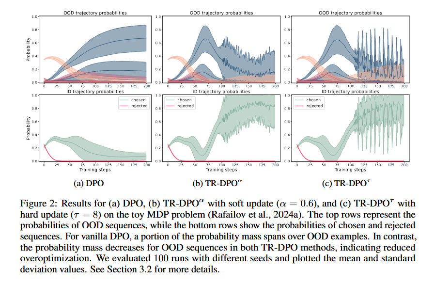
Offline alignment methods (e.g., DPO) fine-tune LLMs using pre-constructed datasets without needing explicit reward models. However, they suffer from overoptimization: as the trained policy (\(\pi_\theta\)) deviates too far from the fixed reference policy (\(\pi_{ref}\), typically a supervised fine-tuned model), the quality of generated outputs degrades. This is linked to increased probabilities of out-of-domain (OOD) data and a decline in in-domain (ID) data probabilities.
Overoptimization in offline methods arises due to vanishing curvature in the loss landscape (analyzed via Hessian dynamics), making it hard to reverse declining ID data probabilities. Updating \(\pi_{ref}\) “resets” the optimization process, restoring curvature and preventing OOD drift.
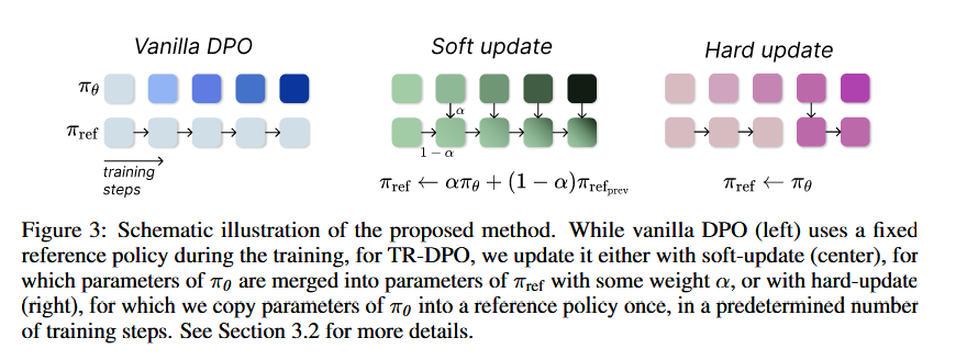
TR-DPO21 address the overoptimization via dynamically updating the reference policy (\(\pi_{ref}\)) during training to mitigate overoptimization. This approach, inspired by trust region optimization, ensures the model stays within a “trustworthy” range of behavior while allowing beneficial divergence from the initial reference. Unlike game-theoretical approaches (which rely on online sampling), TR methods work entirely offline, using pre-existing datasets.
Two update strategies are introduced:
Soft Update: Gradually merges the current policy into the reference policy using a weighted average:
$$\pi_{ref} \leftarrow \alpha \pi_\theta + (1-\alpha) \pi_{ref_{prev}}$$where \(\alpha\) controls the update rate, and stop-gradient (\(sg\)) prevents backpropagating through \(\pi_{ref}\)
Hard Update: Periodically replaces the reference policy with the current policy after a fixed number of steps (\(\tau\)):
$$\pi_{ref} \leftarrow \pi_\theta$$
These strategies are applied to existing methods, creating TR-DPO, TR-IPO, and TR-KTO.
The authors evaluate TR methods on both task-specific and general benchmarks, using models like Pythia (2.8B–12B) and Llama3 (8B):
Task-Specific Tasks:
- On Anthropic-HH (helpful/harmless dialogue) and Reddit TL;DR (summarization), TR methods outperformed vanilla DPO/IPO/KTO. For example, TR-DPO with \(\alpha=0.6\) or \(\tau=512\) achieved 8.4–15% higher win rates.
General Benchmarks:
- On AlpacaEval 2 and Arena-Hard, TR methods showed significant gains. TR-IPO with hard updates improved win rates by 15.1 points on Arena-Hard, while TR-DPO improved by 9.5 points.
Overoptimization Mitigation:
- At equivalent KL divergence (distance from the initial reference), TR methods maintained higher human-centric (HC) metrics (coherence, helpfulness, etc.) compared to vanilla methods, indicating reduced overoptimization.
TR alignment methods (TR-DPO, TR-IPO, TR-KTO) effectively reduce overoptimization by dynamically updating the reference policy. They outperform traditional offline methods across tasks and model sizes, enabling LLMs to diverge beneficially from initial references while maintaining high quality. Future work will explore broader applicability and adaptive update strategies.
Step-DPO: Step-wise Preference Optimization for Long-chain Reasoning
LLMs struggle with long-chain mathematical reasoning due to the need for precise step-by-step correctness. Traditional DPO fails to improve such reasoning effectively because it evaluates entire answers rather than individual steps, making it hard to identify subtle errors in intermediate reasoning.
Step-DPO22 treats each reasoning step as the unit for preference optimization (instead of holistic answers in DPO). By focusing on the first erroneous step in a chain, Step-DPO provides fine-grained supervision, enabling LLMs to locate and correct mistakes more accurately.
Specifically, the answer \( y \) can be decomposed into a sequence of reasoning steps \( y = s_1, \ldots, s_n \), where \( s_i \) is the \( i \)-th reasoning step.
Given a prompt \( x \) and a series of initial correct reasoning steps \( s_{1\sim k-1} = s_1, \ldots, s_{k-1} \), Step-DPO aims to maximize the probability of the correct next reasoning step \( s_{\textit{win}} \) and minimize the probability of the incorrect one \( s_{\textit{lose}} \). This objective can be formulated as:
$$ \mathcal{L}(\theta) = -\mathbb{E}_{(x, s_{1\sim k-1}, s_{\textit{win}}, s_{\textit{lose}}) \sim D} \left[ \log \sigma\left( \beta \log \frac{\pi_\theta(s_{\textit{win}} \mid x; s_{1\sim k-1})}{\pi_{\textit{ref}}(s_{\textit{win}} \mid x; s_{1\sim k-1})} - \beta \log \frac{\pi_\theta(s_{\textit{lose}} \mid x; s_{1\sim k-1})}{\pi_{\textit{ref}}(s_{\textit{lose}} \mid x; s_{1\sim k-1})} \right) \right] $$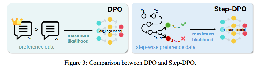
The authors propose a 3-step pipeline to build high-quality step-wise preference data (10K pairs):
- Error Collection: Use a reference model to generate incorrect answers for math problems, retaining cases where the final answer differs from the ground truth.
- Step Localization: Identify the first erroneous step in each incorrect answer manually or with GPT-4.
- Rectification: Generate correct next steps by sampling from the reference model given the initial correct steps, ensuring in-distribution data (self-generated) over out-of-distribution data (human/GPT-4-generated), which proves more effective.
Performance:
- Step-DPO achieves up to 3% accuracy gain on MATH with as few as 10K data pairs and <500 training steps for 70B+ parameter models.
- Qwen2-72B-Instruct + Step-DPO reaches 70.8% on MATH and 94.0% on GSM8K, outperforming closed-source models like GPT-4-1106, Claude-3-Opus, and Gemini-1.5-Pro.
Ablation Studies:
- Step-DPO outperforms DPO by 1.8–2.6% on MATH.
- In-distribution data yields 0.7% higher accuracy than out-of-distribution data.
Identity Preference Optimization (IPO)
RLHF relies on a reward model (via the Bradley-Terry model) that maps pairwise preferences to pointwise rewards (Elo scores), then optimizes the policy using reinforcement learning with KL regularization. However, it suffers from inefficiencies due to reward modeling. DPO avoids reward modeling by directly optimizing the policy from preferences but still relies on the Bradley-Terry assumption. This leads to overfitting, especially when preferences are deterministic (e.g., \( p^{*}(y \succ y') = 1 \)), as the unbounded \(\Psi\) function in its objective ignores KL regularization, pushing the policy to extreme deterministic behavior, leads to policies deviating from the reference policy, even with large regularization parameters.
To unify and address these issues, the Ψ-preference optimization (ΨPO)23 framework, a general objective for preference learning is proposed:
$$ \max_{\pi} \mathbb{E}_{\substack{x \sim \rho \\ y \sim \pi(\cdot|x) \\ y' \sim \mu}} \left[ \Psi\left(p^{*}(y \succ y' | x)\right) \right] - \tau D_{\text{KL}}(\pi \| \pi_{\text{ref}}) $$Here, \(\Psi: [0,1] \to \mathbb{R}\) is a non-decreasing mapping, \(\pi\) is the policy to optimize, \(\mu\) is the behavior policy, \(\pi_{\text{ref}}\) is the reference policy, and \(\tau\) controls KL regularization. RLHF and DPO are shown to be special cases with \(\Psi(q) = \log(q/(1-q))\) (under the Bradley-Terry model).
To avoid overfitting, use a bounded \(\Psi\). A natural choice is the identity mapping (\(\Psi(q) = q\)), leading to the IPO objective:
$$ \max_{\pi} p_{\rho}^{*}(\pi \succ \mu) - \tau D_{\text{KL}}(\pi \| \pi_{\text{ref}}) $$where \( p_{\rho}^{*}(\pi \succ \mu) \) is the total preference of \(\pi\) over \(\mu\). This objective directly optimizes total preferences while retaining effective KL regularization, even for deterministic preferences.
As with DPO, it will be beneficial to re-express IPO objective as an offline learning objective. To derive such an expression.
For the optimal policy \(\pi^*\), the log-likelihood ratio \( h_{\pi}(y, y') = \log\left( \frac{\pi(y) \pi_{\text{ref}}(y')}{\pi(y') \pi_{\text{ref}}(y)} \right) \) must satisfy:
$$ h_{\pi^*}(y, y') = \frac{p^{*}(y \succ \mu) - p^{*}(y' \succ \mu)}{\tau} $$This is rephrased as a loss minimization problem, where the loss \( L(\pi) \) is the expected squared difference between \( h_{\pi}(y, y') \) and the target value above:
$$ L(\pi) = \mathbb{E}_{y, y' \sim \mu} \left[ \left( h_{\pi}(y, y') - \frac{p^{*}(y \succ \mu) - p^{*}(y' \succ \mu)}{\tau} \right)^2 \right] $$To use real-world preference datasets (which contain sampled preferences, not \( p^{*} \)), the paper shows that the theoretical loss can be approximated using empirical data. For a dataset \( D \) of preferred (\( y_w \)) and dispreferred (\( y_l \)) pairs, define \( I(y, y') = 1 \) if \( y \succ y' \) and \( 0 \) otherwise (sampled from a Bernoulli distribution with mean \( p^{*}(y \succ y') \)).
Proposition 3 demonstrates that the empirical loss (using \( I(y, y') \)) is equivalent to the theoretical loss (up to a constant). Exploiting symmetry in \( D \) (each \( (y_w, y_l) \) contributes \( (y_w, y_l, 1) \) and \( (y_l, y_w, 0) \)), the empirical loss simplifies to:
$$ \mathbb{E}_{(y_w, y_l) \sim D} \left[ \left( h_{\pi}(y_w, y_l) - \frac{\tau^{-1}}{2} \right)^2 \right] $$Combining these insights, the Sampled IPO Algorithm is defined as:
- Define \( h_{\pi}(y, y', x) \) for context \( x \): $$ h_{\pi}(y, y', x) = \log\left( \frac{\pi(y|x) \pi_{\text{ref}}(y'|x)}{\pi(y'|x) \pi_{\text{ref}}(y|x)} \right) $$
- Optimize the policy starting from \(\pi_{\text{ref}}\) by minimizing the empirical loss: $$ \min_{\pi} \mathbb{E}_{(y_w, y_l, x) \sim D} \left[ \left( h_{\pi}(y_w, y_l, x) - \frac{\tau^{-1}}{2} \right)^2 \right] $$
In other words IPO, unlike DPO, always regularizes its solution towards $\pi_{\text{ref}}$ by controlling the gap between the log-likelihood ratios $\log(\pi(y_w)/\pi(y_l))$ and $\log(\pi_{\text{ref}}(y_w)/\pi_{\text{ref}}(y_l))$, thus avoiding the over-fitting to the preference dataset.
# ... calculate logits the same as DPO
# https://github.com/huggingface/trl/blob/2c49300910e55fd7482ad80019feee4cdaaf272c/trl/trainer/dpo_trainer.py#L974
# eqn (17) of the paper where beta is the regularization parameter for the IPO loss, denoted by tau in the paper.
losses = (logits - 1 / (2 * self.beta)) ** 2
SPPO - Self-Play Preference Optimization for Language Model Alignment
Paper: Wu, Yue, et al. Self-Play Preference Optimization for Language Model Alignment. arXiv:2405.00675, arXiv, 4 Oct. 2024. arXiv.org, https://doi.org/10.48550/arXiv.2405.00675.
DMPO: Direct Multi-Turn Preference Optimization
Extends DPO to multi-turn dialogue by optimizing preferences across conversation history, improving coherence and relevance in multi-step interactions.
Paper: Shi, Wentao, et al. Direct Multi-Turn Preference Optimization for Language Agents. arXiv:2406.14868, arXiv, 23 Feb. 2025. arXiv.org, https://doi.org/10.48550/arXiv.2406.14868.
WPO - Enhancing RLHF with Weighted Preference Optimization
IV. Reference-Free Optimization
Odds Ratio Preference Optimization (ORPO)
ORPO (Odds Ratio Preference Optimization) combines SFT and preference optimization in a single monolithic training stage, eliminating reference model requirements. This approach streamlines training while maintaining competitive performance across multiple benchmarks.
Paper: Hong, S., et al. (2024). ORPO: Monolithic Preference Optimization without Reference Model.
Existing methods like RLHF and DPO often require:
- A supervised fine-tuning (SFT) warm-up stage.
- A reference model for comparison.
- Complex multi-stage processes, which are resource-intensive.
The core insight: SFT can be enhanced to directly incorporate preference alignment by penalizing undesired generation styles, eliminating the need for extra stages or reference models.
ORPO Algorithm

ORPO integrates preference alignment into SFT using an odds ratio to contrast favored (\(y_w\)) and disfavored (\(y_l\)) responses. The key components are:
- Objective Function: \(\mathcal{L}_{ORPO} = \mathcal{L}_{SFT} + \lambda \cdot \mathcal{L}_{OR}\), where:
- \(\mathcal{L}_{SFT}\) is the standard negative log-likelihood (NLL) loss for SFT.
- \(\mathcal{L}_{OR}\) is a new loss term that maximizes the odds ratio between \(y_w\) and \(y_l\), defined as: \[ \mathcal{L}_{OR} = -\log \sigma\left(\log \frac{odds_\theta(y_w|x)}{odds_\theta(y_l|x)}\right) \] where \(odds_\theta(y|x) = \frac{P_\theta(y|x)}{1-P_\theta(y|x)}\) and \(\sigma\) is the sigmoid function.
- Gradient Analysis: The gradient of \(\mathcal{L}_{OR}\) dynamically penalizes disfavored responses, accelerating adaptation to desired styles while preserving domain knowledge from SFT.
Implementation from https://github.com/huggingface/trl/blob/2c49300910e55fd7482ad80019feee4cdaaf272c/trl/trainer/orpo_trainer.py#L623
def odds_ratio_loss(
        self,
        policy_chosen_logps: torch.FloatTensor,
        policy_rejected_logps: torch.FloatTensor,
    ) -> tuple[torch.FloatTensor, torch.FloatTensor, torch.FloatTensor, torch.FloatTensor, torch.FloatTensor]:
        """Compute ORPO's odds ratio (OR) loss for a batch of policy and reference model log probabilities.

        Args:
            policy_chosen_logps: Log probabilities of the policy model for the chosen responses. Shape: (batch_size,)
            policy_rejected_logps: Log probabilities of the policy model for the rejected responses. Shape: (batch_size,)

        Returns:
            A tuple of three tensors: (losses, chosen_rewards, rejected_rewards).
            The losses tensor contains the ORPO loss for each example in the batch.
            The chosen_rewards and rejected_rewards tensors contain the rewards for the chosen and rejected responses, respectively.
            The log odds ratio of the chosen responses over the rejected responses ratio for logging purposes.
            The `log(sigmoid(log_odds_chosen))` for logging purposes.
        """

        # Derived from Eqs. (4) and (7) from https://huggingface.co/papers/2403.07691 by using log identities and exp(log(P(y|x)) = P(y|x)
        log_odds = (policy_chosen_logps - policy_rejected_logps) - (
            torch.log1p(-torch.exp(policy_chosen_logps)) - torch.log1p(-torch.exp(policy_rejected_logps))
        )
        ratio = F.logsigmoid(log_odds)
        losses = self.beta * ratio

        chosen_rewards = self.beta * (policy_chosen_logps.to(self.accelerator.device)).detach()
        rejected_rewards = self.beta * (policy_rejected_logps.to(self.accelerator.device)).detach()

        return losses, chosen_rewards, rejected_rewards, torch.mean(ratio), torch.mean(log_odds)
Advantages over Existing Methods**
- Monolithic Design: ORPO performs preference alignment in a single stage during SFT, unlike RLHF/DPO’s multi-stage workflows.
- No Reference Model: Avoids the need for a frozen SFT model, reducing memory usage and computational cost (half the forward passes per batch).
- Stability with Odds Ratio: Compared to probability ratios, the odds ratio provides a milder penalty, preventing over-suppression of disfavored responses (Figure 6).
SimPO: Simple Preference Optimization with a Reference-Free Reward
SimPO aligns the reward function with the generation metric, eliminates the need for a reference model, and introduces a target reward margin to enhance performance.
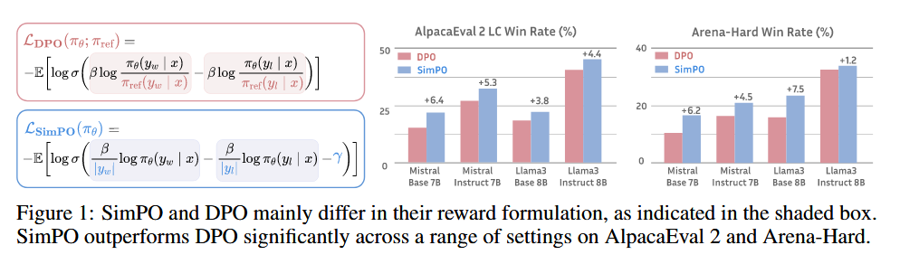
In DPO, for any triple $(x, y_w, y_l)$, satisfying the reward ranking $r(x, y_w) > r(x, y_l)$ does not necessarily gaurantee the likelihood ranking $p_\theta(y_w \mid x) > p_\theta(y_l \mid x)$. The paper found that only roughly 50% of the triples from a held-out set satisfy this condition when trained with DPO.
Paper: SimPO: Simple Preference Optimization with a Reference-Free Reward.
Length-Normalized Reward formulation: Replacing the reward formulation in DPO with $p_\theta$ in the average log likelihood
$$ p_\theta(y \mid x) = \frac{1}{|y|} \log \pi_\theta(y \mid x) = \frac{1}{|y|} \sum_{i=1}^{|y|} \log \pi_\theta(y_i \mid x, y_{\lt i}). $$so that it aligns with the likelihood metric that guides generation, results in a length-normalized reward:
$$ r_{\text{SimPO}}(x, y) = \frac{\beta}{|y|} \log \pi_\theta(y \mid x) = \frac{\beta}{|y|} \sum_{i=1}^{|y|} \log \pi_\theta(y_i \mid x, y_{\lt i}) $$where $\beta$ is a constant that controls the scaling of the reward difference.
This reward eliminates the need for a reference model, enhancing memory and computational efficiency.
Removing the length normalization term from the reward formulation results in a bias toward generating longer but lower-quality sequences.
Target Reward Margin: SimPO incorporates a target margin $\gamma$ into the Bradley-Terry objective to ensure the reward difference between winning ($y_w$) and losing ($y_l$) responses exceeds $\gamma$:
$$ \mathcal{L}_{\text{SimPO}} = -\mathbb{E}\left[\log \sigma\left(\frac{\beta}{|y_w|}\log\pi_{\theta}(y_w|x) - \frac{\beta}{|y_l|}\log\pi_{\theta}(y_l|x) - \gamma\right)\right] $$This margin enhances the model’s ability to distinguish between high-quality and low-quality responses, improving generalization.
The comparison of SimPO with other offline preference optimization methods:
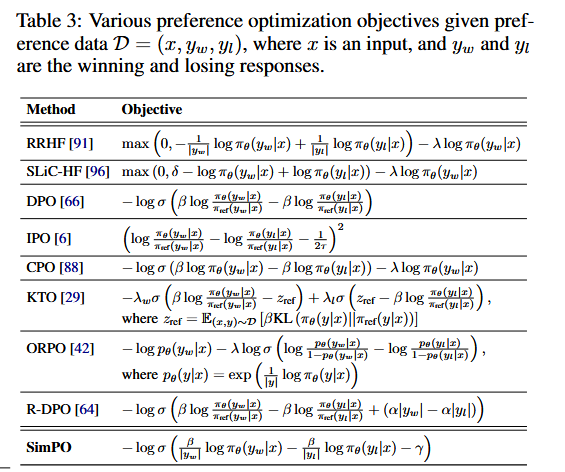
- RRHF and SLiC-HF are ranking losses. RRHF uses length-normalized log-likelihood, similar to SimPO’s reward function, while SLiCHF uses log-likelihood directly and includes an SFT objective.
- IPO is a theoretically grounded approach method that avoids DPO’s assumption that pairwise preferences can be replaced with pointwise rewards.
- CPO uses sequence likelihood as a reward and trains alongside an SFT objective.
- KTO learns from non-paired preference data.
- ORPO introduces a reference-model-free odd ratio term to directly contrast winning and losing responses with the policy model and jointly trains with the SFT objective.
- R-DPO is a modified version of DPO that includes an additional regularization term to prevent exploitation of length.
This paper thoroughly tune the hyperparameters for each baseline and report the best performance. They find that many variants of DPO do not empirically present an advantage over standard DPO.
Implementation: https://docs.pytorch.org/torchtune/0.3/_modules/torchtune/rlhf/loss/dpo.html#SimPOLoss.forward
def simpo_loss(
    policy_chosen_logps: torch.FloatTensor,
    policy_rejected_logps: torch.FloatTensor,
    simpo_gamma,
    beta
):
    logits = (policy_chosen_logps - policy_rejected_logps)
    gamma_logratios = simpo_gamma / beta
    logits = logits - gamma_logratios
    losses = (
        -F.logsigmoid(beta * logits) * (1 - label_smoothing)
        - F.logsigmoid(beta * logits) * label_smoothing
    )
    return losses
V. Non-preference-based methods
KTO - Model Alignment as Prospect Theoretic Optimization
The paper introduces Kahneman-Tversky Optimization (KTO), a approach maximizes the utility of generations instead of maximizing the log-likelihood of preferences(as DPO does).
Theoretically, KTO align LLM with human preferences by framing alignment as a problem of prospect theoretic optimization. Drawing from Kahneman and Tversky’s prospect theory, which describes how humans make decisions under uncertainty with biases like loss aversion, the authors argue that existing alignment methods (e.g., DPO, PPO) implicitly incorporate these biases. They formalize these as Human-Aware Losses (HALOs) and propose KTO as a principled HALO that directly maximizes human utility rather than the log-likelihood of preferences.
Paper: KTO: Model Alignment as Prospect Theoretic Optimization.
KTO Method:
- Derives a HALO using Kahneman-Tversky’s value function, replacing exponents with logistic functions for stability.
- Requires only binary feedback (desirable/undesirable) instead of preference pairs, making data collection cheaper and more scalable.
- Introduces hyperparameters β (risk aversion) and λ_D/λ_U (loss aversion for desirable/undesirable outputs) to model human decision biases.
Prospect Theory in Alignment:
- Value Function: Models human utility relative to a reference point, with concavity in gains and steeper slopes in losses (loss aversion).
- Reference Point: In KTO, the reference is the KL divergence between the current policy and the reference model, estimated via microbatch mismatches for stability.
Loss Function:
$\lambda_y$ denotes $\lambda_D$ ($\lambda_U$) when $y$ is desirable(undesirable) respectively, the default KTO loss is:
$$ \mathcal{L}_{\text{KTO}}(\pi_\theta, \pi_{\text{ref}}) \triangleq \mathbb{E}_{x,y \sim D} \left[ \lambda_y - v(x,y) \right] \tag{8} $$where
$$ r_\theta(x,y) = \log \frac{\pi_\theta(y|x)}{\pi_{\text{ref}}(y|x)}, $$$$ z_0 = \text{KL}\bigl(\pi_\theta(y'|x) \big\| \pi_{\text{ref}}(y'|x)\bigr), $$$$ v(x,y) = \begin{cases} \lambda_D \sigma\bigl(\beta(r_\theta(x,y) - z_0)\bigr) & \text{if } y \sim y_{\text{desirable}}|x, \\ \lambda_U \sigma\bigl(\beta(z_0 - r_\theta(x,y))\bigr) & \text{if } y \sim y_{\text{undesirable}}|x. \end{cases} $$Implementation from https://github.com/huggingface/trl/blob/2c49300910e55fd7482ad80019feee4cdaaf272c/trl/trainer/kto_trainer.py#L1090:
def kto_loss(
        policy_chosen_logps: torch.FloatTensor,
        policy_rejected_logps: torch.FloatTensor,
        policy_KL_logps: torch.FloatTensor,
        reference_chosen_logps: torch.FloatTensor,
        reference_rejected_logps: torch.FloatTensor,
        reference_KL_logps: torch.FloatTensor,
    ):
    kl = (policy_KL_logps - reference_KL_logps).mean().detach()
    # Chosen losses
    if policy_chosen_logps.shape[0] != 0 or reference_chosen_logps.shape[0] != 0:
        chosen_logratios = policy_chosen_logps - reference_chosen_logps
        chosen_losses = 1 - F.sigmoid(beta * (chosen_logratios - kl))
        chosen_rewards = beta * chosen_logratios.detach()
    else:
        chosen_losses = torch.Tensor([])
        chosen_rewards = torch.Tensor([])

    # Rejected losses
    if policy_rejected_logps.shape[0] != 0 or reference_rejected_logps.shape[0] != 0:
        rejected_logratios = policy_rejected_logps - reference_rejected_logps
        rejected_losses = 1 - F.sigmoid(beta * (kl - rejected_logratios))
        rejected_rewards = beta * rejected_logratios.detach()
    else:
        rejected_losses = torch.Tensor([])
        rejected_rewards = torch.Tensor([])

    losses = torch.cat(
        (chosen_losses, rejected_losses),
        0,
    )
    return losses
VI. Others
SPO - A Minimaximalist Approach to Reinforcement Learning from Human Feedback
Uses self-play to generate preference data, where models compete to maximize rewards. It employs a minimax approach to balance exploration and exploitation. Paper: A Minimaximalist Approach to Reinforcement Learning from Human Feedback.
VII. Key Trends and Challenges
[]: https://github.com/volcengine/verl
- Scalability: Methods like RLHF and DPO face challenges with large models (e.g., 405B parameters) due to memory and computational costs. Frameworks like Verl address this via asynchronous distributed training .
- Data Efficiency: SimPO and ORPO reduce reliance on reference models and pairwise data, while Step-DPO and KTO focus on fine-grained optimization .
- Generalization: SPO and DMPO aim to improve generalization across tasks (e.g., dialogue, math) by leveraging self-play and multi-turn optimization .
- Theoretical Foundations: KTO and SimPO provide theoretical insights into preference learning, linking RL to prospect theory and information theory .
VIII. Future Directions
- Multi-Modality: IPO and DMPO highlight the need for alignment across text, video, and dialogue.
- Self-Supervised Learning: RLAIF and SPO explore AI-generated feedback to reduce human labeling.
- Efficiency: …
Schulman, John, et al. Proximal Policy Optimization Algorithms. arXiv:1707.06347, arXiv, 28 Aug. 2017. arXiv.org, http://arxiv.org/abs/1707.06347. ↩︎
Ouyang, Long, et al. Training Language Models to Follow Instructions with Human Feedback. arXiv:2203.02155, arXiv, 4 Mar. 2022. arXiv.org, http://arxiv.org/abs/2203.02155. ↩︎
Bai, Yuntao, et al. Constitutional AI: Harmlessness from AI Feedback. arXiv:2212.08073, arXiv, 15 Dec. 2022. arXiv.org, https://doi.org/10.48550/arXiv.2212.08073. ↩︎
Lee, Harrison, et al. RLAIF vs. RLHF: Scaling Reinforcement Learning from Human Feedback with AI Feedback. arXiv:2309.00267, arXiv, 3 Sept. 2024. arXiv.org, https://doi.org/10.48550/arXiv.2309.00267. ↩︎
Shao, Zhihong, et al. DeepSeekMath: Pushing the Limits of Mathematical Reasoning in Open Language Models. arXiv:2402.03300, arXiv, 27 Apr. 2024. arXiv.org, http://arxiv.org/abs/2402.03300. ↩︎
J. Schulman. Approximating kl divergence, 2020. URL http://joschu.net/blog/kl-approx.html. ↩︎
DeepSeek-AI, et al. DeepSeek-R1: Incentivizing Reasoning Capability in LLMs via Reinforcement Learning. arXiv:2501.12948, arXiv, 22 Jan. 2025. arXiv.org, https://doi.org/10.48550/arXiv.2501.12948. ↩︎
Ahmadian, Arash, et al. Back to Basics: Revisiting REINFORCE Style Optimization for Learning from Human Feedback in LLMs. arXiv:2402.14740, arXiv, 26 Feb. 2024. arXiv.org, https://doi.org/10.48550/arXiv.2402.14740. ↩︎
https://huggingface.co/blog/putting_rl_back_in_rlhf_with_rloo ↩︎
Huang, Shengyi, et al. A2C Is a Special Case of PPO. arXiv:2205.09123, arXiv, 18 May 2022. arXiv.org, https://doi.org/10.48550/arXiv.2205.09123. ↩︎
Li, Ziniu, et al. ReMax: A Simple, Effective, and Efficient Reinforcement Learning Method for Aligning Large Language Models. arXiv:2310.10505, arXiv, 16 May 2024. arXiv.org, https://doi.org/10.48550/arXiv.2310.10505. ↩︎ ↩︎
https://hijkzzz.notion.site/unraveling-rlhf-and-its-variants-engineering-insights ↩︎
Hu, Jian, et al. REINFORCE++: An Efficient RLHF Algorithm with Robustness to Both Prompt and Reward Models. arXiv:2501.03262, arXiv, 6 Apr. 2025. arXiv.org, https://doi.org/10.48550/arXiv.2501.03262. ↩︎
Yu, Qiying, et al. DAPO: An Open-Source LLM Reinforcement Learning System at Scale. arXiv:2503.14476, arXiv, 20 May 2025. arXiv.org, https://doi.org/10.48550/arXiv.2503.14476. ↩︎
Liu, Zichen, et al. Understanding R1-Zero-Like Training: A Critical Perspective. arXiv:2503.20783, arXiv, 26 Mar. 2025. arXiv.org, https://doi.org/10.48550/arXiv.2503.20783. ↩︎
Feng, Lang, et al. Group-in-Group Policy Optimization for LLM Agent Training. arXiv:2505.10978, arXiv, 16 May 2025. arXiv.org, https://doi.org/10.48550/arXiv.2505.10978. ↩︎
Zheng, Chujie, et al. “Group Sequence Policy Optimization.” arXiv:2507.18071, arXiv, 28 July 2025. arXiv.org . ↩︎
Direct Preference Optimization: Your Language Model is Secretly a Reward Model. ↩︎
Guo, Shangmin, et al. Direct Language Model Alignment from Online AI Feedback. arXiv:2402.04792, arXiv, 29 Feb. 2024. arXiv.org, https://doi.org/10.48550/arXiv.2402.04792. ↩︎
Gorbatovski, Alexey, et al. Learn Your Reference Model for Real Good Alignment. arXiv:2404.09656, arXiv, 25 Feb. 2025. arXiv.org, https://doi.org/10.48550/arXiv.2404.09656. ↩︎
Lai, Xin, et al. Step-DPO: Step-Wise Preference Optimization for Long-Chain Reasoning of LLMs. arXiv:2406.18629, arXiv, 26 Jun. 2024. arXiv.org, https://doi.org/10.48550/arXiv.2406.18629. ↩︎
Azar, Mohammad Gheshlaghi, et al. A General Theoretical Paradigm to Understand Learning from Human Preferences. arXiv:2310.12036, arXiv, 21 Nov. 2023. arXiv.org, http://arxiv.org/abs/2310.12036. ↩︎