Combining reinforcement learning and deep neural networks at scale. The algorithm was developed by enhancing a classic RL algorithm called Q-Learning with deep neural networks and a technique called experience replay.
Q-Learning
Q-Learning is based on the notion of a Q-function. The Q-function (a.k.a the state-action value function) of a policy $\pi$,$Q^{\pi}(s, a)$ ,measures the expected return or discounted sum of rewards obtained from state $s$ by taking action $a$ first and following policy $\pi$ thereafter.
The optimal Q-function $Q^{*}(s, a)$ obeys the following Bellman optimality equation:
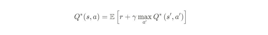
This means that the maximum return from state s and action a is the sum of the immediate reward $r$ and the return (discounted by $\gamma$) obtained by following the optimal policy thereafter until the end of the episode(i.e., the maximum reward from the next state $s^{\prime}$). The expectation is computed both over the distribution of immediate rewards $r$ and possible next states $s^{\prime}$.
Each sequence from the initial state and action to the end is called an episode.
通过期望值来预估未来状态
假设没有$\gamma$ ,那么未来长期reward没有折损,会得到 sparse reward:因为没有折损,所有状态最后得到的值是一样的,模型无法获得差异信号
- It is important to tune this hyperparameter to get optimum results.
- Successful values range from 0.9 to 0.99.
- A lower value encourages short-term thinking
- A higher value emphasizes long-term rewards
The Bellman Equation was introduced by Dr. Richard Bellman (who’s known as the Father of dynamic programming) in 1954 in the paper: The Theory of Dynamic Programming.
Use the Bellman optimality equation as an iterative update
$$Q_{i + 1}(s, a) \leftarrow E\left[r+\gamma \max_{a^{\prime}} Q_{i}(s^{\prime}, a^{\prime})\right]$$this converges to the optimal Q-function, i.e $Q_{i} \rightarrow Q^{*} \text { as } i \rightarrow \infty$
在深度学习之前,Bellman optimality equation 使用递归求解,在每层递归中,需要知道能使预期长期回报最大化的最佳操作是什么。也就是会遍历庞大的递归搜索树。
在Non-deterministic情况下,BO函数变成
$$Q(s, a) = R(s, a) + \gamma \sum_{s'}P(s, a, s') max_{a'}Q(s', a'))$$Temporal Difference
Non-deterministic search can be very difficult to actually calculate the value of each state.
用Temporal difference 来迭代更新每一个事件的Q-value. $\alpha$是学习率
$$Q_t(s, a) = Q_{t-1}(s, a) + \alpha TD_t(a, s)$$假设t时间步选择了$(s', a')$,则Temporal difference是
$$TD(a, s) = R(s, a) + \gamma max_{a'}Q(s', a') - Q_{t-1}(s, a)$$由于Non-deterministic环境中存在的随机性,TD值一般不会为0,就可以随着每一时间步的推进更新Q-value
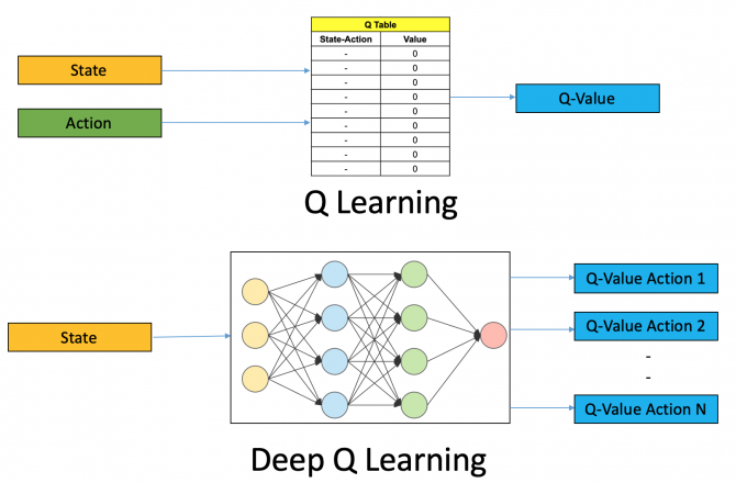
Deep Q-Learning
For most problems, it is impractical to represent the Q-function as a table containing values for each combination of s and a. Instead, we train a function approximator, such as a neural network with parameters $\theta$, to estimate the Q-values, i.e. $Q(s, a ; \theta) \approx Q^{*}(s, a)$, by minimizing the following loss at each step i:

其中 $y_i$是TD Target, $y_i - Q$ is the TD error. $s, a, r, s^{\prime}$是可能的状态转移
Note that the parameters from the previous iteration $\theta_{i-1}$ are fixed and not updated. In practice we use a snapshot of the network parameters from a few iterations ago instead of the last iteration. This copy is called the target network.
https://www.analyticsvidhya.com/blog/2019/04/introduction-deep-q-learning-python/
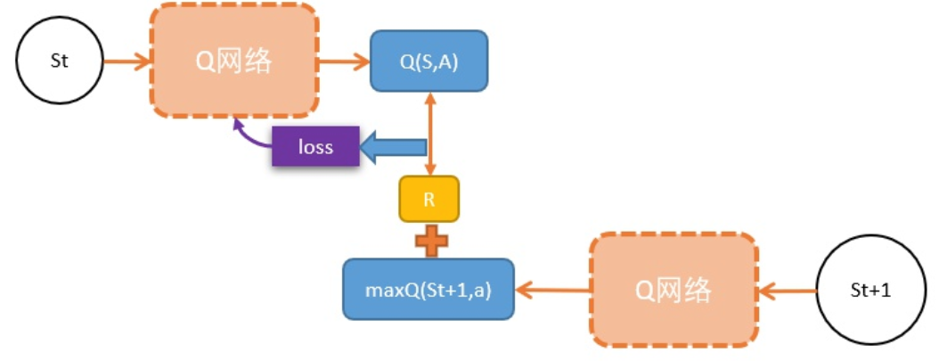
初始化一个网络,用于计算Q值,假设当前状态St,
- 把St输入到Q,计算该状态下,各个动作的Q值 $Q(s)$
- 选择能得到最大Q值的动作A, 需要更新当前状态St下的动作A的Q值:$Q(S,A)$,
- 执行A,输入到环境,往前一步,到达St+1;
- 把St+1输入Q网络,计算St+1下所有动作的Q值;
- 获得最大的Q值,用gamma 折损,加上奖励R作为更新目标;
- 计算损失
Q(S,A)相当于有监督学习中的logitsgamma * maxQ(St+1) + R相当于有监督学习中的lables- 用mse函数,得出两者的loss
- 用loss更新Q网络,缩小
Q(S,A)和目标。
不断循环以上步骤
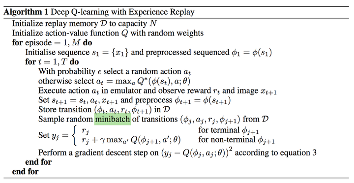
Experience Replay
经验池的技巧,就是如何存储样本及采样问题。由于玩Atari采集的样本是一个时间序列,样本之间具有连续性,如果每次得到样本就更新Q值,受样本分布影响,效果会不好。因此,一个很直接的想法就是把样本先存起来,然后随机采样如何?这就是Experience Replay的意思。按照脑科学的观点,人的大脑也具有这样的机制,就是在回忆中学习。
反复试验,然后存储数据。数据存到一定程度,就每次随机采用数据,进行梯度下降!在DQN中增强学习Q-Learning算法和深度学习的SGD训练是同步进行的,通过Q-Learning获取无限量的训练样本,然后对神经网络进行训练。
Action Selection Policies
once we have the Q-values, how do decide which one to use?
Recall that in simple Q-learning we just choose the action with the highest Q-value. With deep Q-learning we pass the Q-values through a softmax function. The reason that we don’t just use the highest Q-value comes down to an important concept in reinforcement learning: the exploration vs. exploitation dilemma.
there are others that could be used, and a few of the most common include:
- ϵ greedy: selects the greedy action with probability 1- ϵ, and a random action with probability ϵ to ensure good coverage of the state-action space.
- ϵ soft
- Softmax