爱丁堡大学信息学院课程笔记 Accelerated Natural Language Processing, Informatics, University of Edinburgh
References: Accelerated natural language processing ANLP revision guide Lecture Slides from the Stanford Coursera course Natural Language Processing, by Dan Jurafsky and Christopher Manning
概率模型 Probability Model
概率模型是随机现象的数学表示,由样本空间,样本空间内的事件以及与每个事件相关的概率定义。目标是模拟给一个事件发生的概率
估算概率(Probability Estimation)一般使用最大似然估计(MLE,相关频率):
$$p(x_i) = \frac{Count(x_i)}{\sum_{i=0}^nCount(x_i)}$$平滑Smoothing
一般用于处理0概率的问题,比如在训练集中看不到, 但出现在测试集中的词。
Language modeling
To compute the probability of sentence /sequence of words $P(w_1, w_2, w_3...)$, or to predict upcomming words $P(w|w_1, w_2, w_3...)$… a language model is also a probability model.
Probability computation makes use of chain rule of probability, the products of a sequence of conditional probability.
$$P(w_{1:n}) = P(w_1)P(w_2|w_1)P(w_3|w_{1:2})P(w_4|w_{1:3})...P(w_n|w_{1:n-1})$$But the last term based on the entire sentence is very difficult to compute. So it is simplified by Markov Assumption: approximate the conditional probability by only accounting several prefixes, a one-order Markov assumption simplifies as P(the| water is so transparent that) ≈ P(the| that)
Evaluation: Perplexity
Perplexity
Intuition based on Shannon game: The best language model is one that best predicts an unseen test set(e.g. next word), gives the highest $P(sentence)$ to the word that actually occurs.
- Definition: Perplexity is the inverse probability of the test set, normalized by the number of words(lie between 0-1).
Normalize the log probability of all the test sentences:
$$\frac{1}{M} \log_2 \prod_{i=1}^m p(x^{(i)}) = \frac{1}{M} \sum_{i=1}^m \log_2 p(x^{(i)})$$Then transform to perplexity:
$$Perplexity = 2^{-\frac{1}{M} \sum_{i=1}^m \log_2 p(x^{(i)})}$$So minimizing perplexity is the same as maximizing probability
Bad approximation: unless the test data looks just like the training data, so generally only useful in pilot experiments.
N-Gram Language Model
N-Gram语言模型是基于N-1阶马尔可夫假设且由MLE估算出的LM。N-GramLM 预测下一个单词出现概率仅条件于前面的(N-1)个单词, 以The students opened their books为例:
Bi-gram: 统计$P(w_{i}=m|w_{i-1})$,P(students | the),P(opened | students), …, 属于马尔可夫一阶模型, 即当前t时间步的状态仅跟t-1相关.Tri-gram:P(students | </s> The),P(opened | The students),马尔可夫二阶模型Four-gram: 依此类推
特殊的Uni-gram: 统计$P(w_i)$, P(the), P(students), …, 此时整个模型退化为词袋模型, 不再属于马尔可夫模型, 而是基于贝叶斯假设, 即各个单词是条件独立的. 所以一般N-gram是指N>1的.
How to estimate theparameter? Maximum likelyhood estimate:
$$P(w_{i}=m|w_{i-n:i-1}) = \frac{Count(w_{i-n:i})}{Count(w_{i-n:i-1})}$$In practice, use log space to avoid underflow, and adding is faster than multiplying.
- Insufficient:
- To catch long-distance dependencies, the
nhas to be very large, that asks for very large memory requirement - N-grams only work well for word prediction if the test corpus looks like the training corpus.
- To catch long-distance dependencies, the
- Sparsity:
- Zero count of gram, means zero probability? No. To deal with 0 probability, commonly use Kneser-Ney smoothing, for very large N-grams like web, use stupid backoff.
Add Alpha Smoothing
- Assign equal probability to all unseen events.
- Applied in text classification, or domains where zeros probability is not common.
Backoff Smoothing
- Use information from lower order N-grams (shorter histories)
- Back off to a lower-order N-gram if we have zero evidence for a higher-order interpolation N-gram.
- Discount: In order for a backoff model to give a correct probability distribution, we have to discount the higher-order N-grams to save some probability mass for the lower order N-grams.
Interpolation Smoothing
- Interpolation: mix the probability estimates from all the N-gram estimators, weighing and combining the trigram, bigram, and unigram counts
- Simple interpolation: $P(w_3|w_1, w_2) = \lambda_1 P(w_3|w_1, w_2) + \lambda_2 P(w_3|w_2) + \lambda_3 P(w_3), \sum \lambda = 1$.
- λ could be trianed/conditioned on training set/contest, choose λ that maximie the probability of held-out data
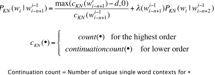
Kneser-Ney Smoothing
- Combine absolute discounting and interpolation: Extending interpolatation with an absolute discounting 0.75 for high order grams.
- Use a better estimate for probabilities of lower-order unigrams, the continuation probability, $P_{continuatin}(w)$ is how likely is w to appear as a novel continutaion.
- For each word w, count the number of bigram types it completes. Or count the number of word types seen to precede w.
- Every bigram type was a novel continuation the first time it was seen.
- normalized by the total number of word bigram types.
- To lower the probability of some fix bigram like “San Franscio”
- For general N-gram,
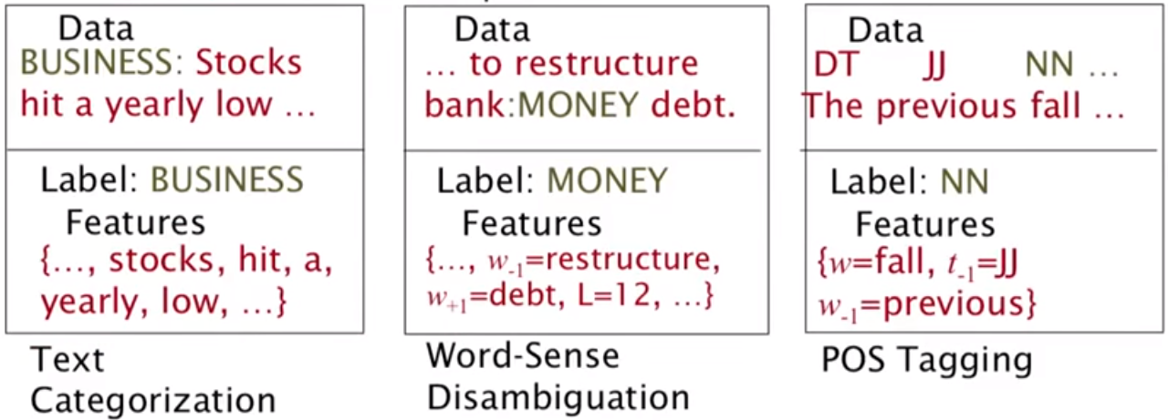
Naive Bayes Classifier
- Application: Text classification, to classify a text, we calculate each class probability given the test sequence, and choose the biggest one.
- Evaluation: precision, recall, F-measure
- Strength and Weakness: 高效, 快速, 但对于组合性的短语词组, 当这些短语与其组成成分的字的意思不同时, NB的效果就不好了
Text Classification
Or text categorization, method is not limited to NB, see lab7. Spam email, gender/authorship/language identification, sentiments analysis,(opinion extraction, subjectivity analysis)…
Sentiments Analysis
- For sentiment(or other text classification), word occurrence may matter more than word frequency. Thus it often improves performance to clip the word counts in each document at 1.
- This variant binary NB is called binary multinominal naive Bayes or binary NB.
- Remove duplicates in each data sample - bag of words representation, boolean features. Binarized seems to work better than full word counts.
- Deal with negation:
like, not like, A very simple baseline that is commonly used in sentiment to deal with negation is during text normalization to prepend the prefix NOT_ to every word after a token of logical negation - Sentiment lexicons: lists of words that are preannotated with positive or negative sentiment. To deal with insufficient labeled training data. A common way to use lexicons in the classifier is to use as one feature the total count of occurrences of any words in the positive lexicon, and as a second feature the total count of occurrences of words in the negative lexicon. Using just two features results in classifiers that are much less sparse to small amounts of training data, and may generalize better. See lab8.
Naive Bayes Assumptions
- Bags of words: a set of unordered words/features with its frequency in the documents, their order was ignored.
- Conditional independence: the probabilities $P(w|C)$ are independence given the class, thus a sequence of words(w1,w2,w3…) probability coculd be estimate via prducts of each $P(w_i|C)$ by walking through every pisition of the sequence, noted that the orders in the sequence does not matter.
Naive Bayes Training
- Each classes’ prior probability P(C) is the percentage of the classes in the training set.
- For the test set, its probability as a class j, is the products of its sequence probability $P(w_1, w_2, w_3...|C_j)$ and $P(C_j)$, normalized by the sequence probability $P(w_1, w_2, w_3...)$, which could be calculated by summing all $P(w_1, w_2, w_3...|C_j)\*P(C_j)$.
- The joint features probability $P(w_1, w_2, w_3...|C)$ of each class is calculated by naively multiplying each word’s MLE given that class.
- In practice, to deal with 0 probability, we dun use MLE, instead we use add alpha smoothing.
- Why 0 probability matters? Because it makes the whole sequence probability $P(w_1, w_2, w_3...|C)$ 0, then all the other features as evidence for the class are eliminated too.
- How: first extract all the vocabulary V in the training set.
- Then, for each feature/word k, its add alpha smoothing probability estimation within a class j is $(Njk + \alpha)/(N_j+V\*\alpha)$.
- This is not the actual probability, but just the numerator.
Naive Bayes Relationship to Language Modelling
- When using all of the words as features for naive bayes, then each class in naive bayes is a unigram languange model.
- For each word, assign probability $P(word|C)$,
- For each sentence, assign probability $P(S|C) = P(w_1, w_2, w_3...|C)$
- Running multiple languange models(classes) to assign probabilities, and pick out the highest language model.
Hidden Markov Model
The HMM is a probabilistic sequence model: given a sequence of units (words, letters, morphemes, sentences, whatever), they compute a probability distribution over possible sequences of labels and choose the best label sequence.
HMM参数$λ= (Y, X, π, A, B)$ :
- Y是隐状态(输出变量)的集合
- X是观察值(输入)集合
- Initial probability π
- Transition probability matrix A, $P(Tag_{i+1} | Tag_{i})$
- Emission probability B, $P(Word | Tag)$
Application: part-of-speech tagging, name entity recognition(NEr), parse tree, speech recognition
Hidden?: these tags, trees or words is not observed(hidden). b比如在POS任务中, X就是观察到的句子, Y就是待推导的标注序列, 因为词性待求的, 所以人们称之为隐含状态.
The three fundamental problems of HMM:
- decoding: discover the best hidden state sequence via Viterbi algorithm.
- Probability of the observation: Given an HMM with know parameters λ and an observation sequence O, determine the likelihood $P(O| \lambda)$ (a language model regardless of tags) via Forward algorithm
- Learning (training): Given only the observed sequence, learn the best(MLE) HMM parameters λ via forward-backward algorithm, thus training a HMM is an unsupervised learning task.
算法:
- 前向算法和后向算法解决如何计算似然$P(O| \lambda)$的问题
- Viterbi算法解决HMM 解码问题.
- 这些算法都是动态规划算法
HMM的缺陷是其基于观察序列中的每个元素都相互条件独立的假设。即在任何时刻观察值仅仅与状态(即要标注的标签)有关。对于简单的数据集,这个假设倒是合理。但大多数现实世界中的真实观察序列是由多个相互作用的特征和观察序列中较长范围内的元素之间的依赖而形成的。而条件随机场(conditional random fiel, CRF)恰恰就弥补了这个缺陷.
同时, 由于生成模型定义的是联合概率,必须列举所有观察序列的可能值,这对多数领域来说是比较困难的。
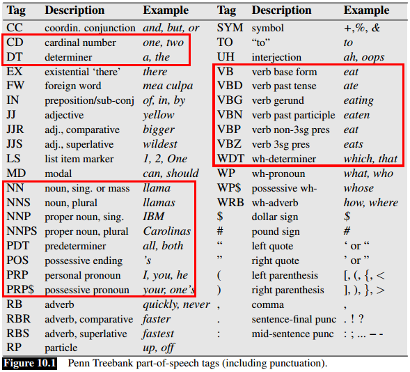
Part-of-speech Tagging
- Part-of-speech(POS), word classes, or syntactic categories, a description of eight parts-of-speech: noun, verb, adjective, adverb, pronoun, preposition, conjunction, interjection, and sometimes numeral, article or determiner.
- noun 名詞 (代號 n. )
- pronoun 代名詞 (代號 pron. )
- verb 動詞 (代號 v. )
- adjective 形容詞 (代號 adj. )
- adverb 副詞 (代號 adv. )
- preposition 介系詞 (代號 prep. )
- conjunction 連接詞 (代號 conj. )
- interjection 感歎詞 (代號 int. )
- Motivation: Use model to find the best tag sequence T for an untagged sentence S: argmax $P(T|S)$ -> argmax $P(S|T)\*P(T)$, where P(T) is the transition (prior) probabilities, $P(S|T)$ is the emission (likelihood) probabilities.
- Parts-of-speech can be divided into two broad supercategories: closed class types and open class types
- Search for the best tag sequence: Viterbi algorithm
- evaluation: tag accuracy
Transition Probability Matrix
- Tags or states
- Each (i,j) represent the probability of moving from state i to j
- When estimated from sequences, should include beginning
<s>and end</s>markers. - Tag transition probability matrix: the probability of tag i followed by j
Emission Probability
- Also called observation likelihoods, each expressing the probability of an observation j being generated from a states i.
- Word/symbol
Penn Treebank
Forward Algorithm
- Compute the likelihood of a particular observation sequence.
- Implementation is almost the same as Viterbi.
- Yet Viterbi takes the max over the previous path probabilities whereas the forward algorithm takes the sum.
Viterbi Algorithm
Decoding task: the task of determining which sequence of variables is the underlying source of some sequence of observations.
Viterbi的实现参考HMM POS Tagging
Intuition: The probability of words $w_1$ followed by $w_2$ with tag/state i and j (i,j is index of all Tags), is the chain rule of the probability of i followed by j and the probability of i output $w_i$ $P(w_1 | i)$ and $P(w_2 |j)$, then choose the maximum from all the possible i j. Then using chain rule to multiply the whole sequence of words.
The value of each cell $Vt(j)$ is computed by recursively taking the most probable path that could lead us to this cell from left columns to right. See exampls in tutorial 2
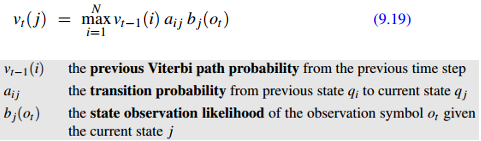
- Since HMM based on Markov Assumptions, so the present column $V_t$ is only related with the nearby left column $V_{t-1}$.
HMM Training
给定观察序列$X = x_1, x_2, ..., x_t$ ,训练调整模型参数λ, 使$p(X | \lambda)$最大: Baum-Welch算法 (Forward-backward algorithm)
- inputs: just the observed sequence
- output: the converged
λ(A,B). - For each interation k until λ converged:
- Compute expected counts using
λ(k-1) - Set
λ(k)using MLE on the expected counts.
- Compute expected counts using
经常会得到局部最优解.
Context-free Grammar
CFG(phrase-structure grammar) consists of a set of rules or productions, each of which expresses the ways that symbols of the language can be grouped and ordered toLexicon gether, and a lexicon of words and symbols.
Constituency
Phrase structure, organizes words into nested constituents. Groups of words behaving as a single units, or constituents.
- Noun phrase(NP), a sequence of words surrounding at least one noun. While the whole noun phrase can occur before a verb, this is not true of each of the individual words that make up a noun phrase
- Preposed or Postposed constructions. While the entire phrase can be placed differently, the individual words making up the phrase cannot be.
- Fallback: In languages with free word order, phrase structure (constituency) grammars don’t make as much sense.
- Headed phrase structure: many phrase has head, VP->VB, NP->NN, the other symbols excepct the head is modifyer.
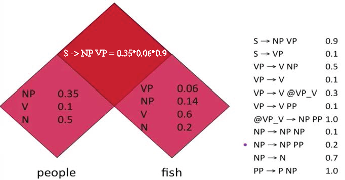
Probabilistic Context-free Grammar
PCFG(Stochastic Context-Free Grammar SCFG (SCFG)), a probabilistic augmentation of context-free grammars in which each rule is associated with a probability.
- G = (T,N,S,R,P)
- T, N: Terminal and Non-terminal
- S: starts symbol
- R: Derive rule/grammar, N -> N/C
- P: a probability function, for a given N, ΣP(N->Ni/Ci)=1. Normally P(S->NP VP)=1, because this is the only rule for S.
- PCFG could generates a sentence/tree,
- thus it is a language model, assigns a probability to the string of words constituting a sentence
- The probability of a tree t is the product of the probabilities of the rules used to generate it.
- The probability of the string s is the sum of the probabilities of the trees/parses which have that string as their yield.
- The probability of an ambiguous sentence is the sum of the probabilities of all the parse trees for the sentence.
- Application: Probabilistic parsing
- Shortage: lack the lexicalization of a trigram model, i.e only a small fraction of the rules contains information about words. To solve this problem, use lexicalized PCFGs
Lexicalization of PCFGs
- The head word of phrase gives a good representation of the phrase’s structure and meaning
- Puts the properties of words back into a PCFG
- Word to word affinities are useful for certain ambiguities, because we know the probability of rule with words and words now, e.g. PP attachment ambiguity
Recursive Descent Parsing
It is a top-down, depth-first parser:
- Blindly expand nonterminals until reaching a terminal (word).
- If multiple options available, choose one but store current state as a backtrack point (in a stack to ensure depth-first.)
- If terminal matches next input word, continue; else, backtrack
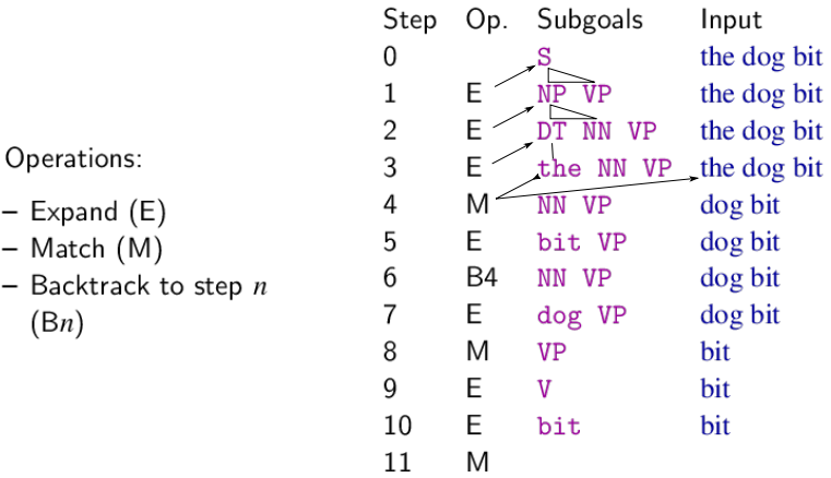
- Can be massively inefficient (exponential in sentence length) if faced with local ambiguity
- Can fall into infinite loop
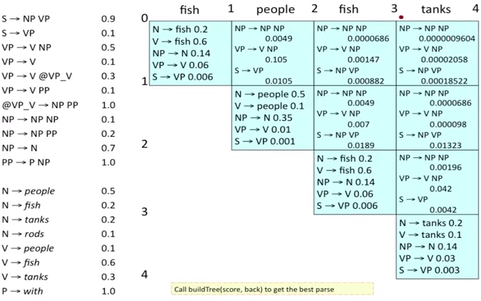
CKY Parsing
Well-formed substring table: For parsing, subproblems are analyses of substrings, memoized in well-formed substring table(WFST, chart).
- Chart entries are indexed by start and end positions in the sentence, and correspond to:
- either a complete constituent (sub-tree) spanning those positions (if working bottom-up),
- or a prediction about what complete constituent might be found (if working top-down).
- The chart is a matrix where cell
[i, j]holds information about the word span from position i to position j:- The root node of any constituent(s) spanning those words
- Pointers to its sub-constituents
- (Depending on parsing method,) predictions about what constituents might follow the substring.
Probability CKY parsing:
Dependency Parsing
- Motivation: context-free parsing algorithms base their decisions on adjacency; in a dependency structure, a dependent need not be adjacent to its head (even if the structure is projective); we need new parsing algorithms to deal with non-adjacency (and with non-projectivity if present).
- Approach: Transition-based dependency parsing
Dependency Syntax
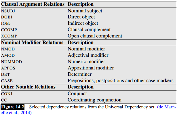
Dependency structure shows which words depend on (modify or are arguments of) which other words.
- A fully lexicalized formalism without phrasal constituents and phrase-structure rules: binary, asymmetric grammatical relations between words.
- More specific, head-dependent relations, with edges point from heads to their dependents.
- Motivation: In languages with free word order, phrase structure (constituency) grammars don’t make as much sense. E.g. we may need both S → NP VP and S → VP NP, but could not tell too much information simply looking at the rule.
- Dependencies: Identifies syntactic relations directly. The syntactic structure of a sentence is described solely in terms of the words (or lemmas) in a sentence and an associated set of directed binary grammatical relations that hold among the words.
- Relation between phrase structure and dependency structure
- Convert phrase structure annotations to dependencies via head rules. (Convenient if we already have a phrase structure treebank.): For a given lexicalized constituency parse(CFG tree), remove the phrasal categories, remove the (duplicated) terminals, and collapse chains of duplicates.
- The closure of dependencies give constituency from a dependency tree
Transition-based Dependency Parsing
transition-based systems use supervised machine learning methods to train classifiers that play the role of the oracle. Given appropriate training data, these methods learn a function that maps from configurations to transition operators(actions).
- Bottom up
- Like shift-reduce parsing, but the ‘reduce’ actions are specialized to create dependencies with head on left or right.
- configuration:consists of a stack, an input buffer of words or tokens, and a set of relations/arcs, a set of actions.
- How to choose the next action: each action is predicted by a discriminative classifier(often SVM, could be maxent) over each legal move.
- features: a sequence of the correct (configuration, action) pairs
f(c ; x).
- features: a sequence of the correct (configuration, action) pairs
- Evaluation: accuracy (# correct dependencies with or ignore label)).
Dependency Tree
- Dependencies from a CFG tree using heads, must be projective: There must not be any crossing dependency arcs when the words are laid out in their linear order, with all arcs above the words.
- But dependency theory normally does allow non-projective structures to account for displaced constituents.
Bounded and Unbounded Dependencies
Unbounded dependency could be considered as long distance dependency
- Long-distance dependencies: contained in wh-non-subject-question, “What flights do you have from Burbank to Tacoma Washington?”, the Wh-NP
what flightsis far away from the predicate that it is semantically related to, the main verbhavein the VP.
Noisy Channel Model:
- The intuition of the noisy channel model is to treat the misspelled word as if a correctly spelled word had been “distorted” by being passed through a noisy communication channel.
- a probability model using Bayesian inference, input -> noisy/errorful encoding -> output, see an observation x (a misspelled word) and our job is to find the word w that generated this misspelled word.
- $P(w|x) = P(x|w)\*P(w)/P(x)$
Noisy channel model of spelling using naive bayes
- The noisy channel model is to maximize the product of likelihood(probability estimation) P(s|w) and the prior probability of correct words P(w). Intuitively it is modleing the noisy channel that turn a correct word ‘w’ to the misspelling.
- The likelihood(probability estimation) P(s|w) is called the the channel/error model, telling if it was the word ‘w’, how likely it was to generate this exact error.
- The P(w) is called the language model
Generative vs. Discriminative Models
Generative(joint) models palce probabilities $p(c, d)$ over both observed data d and the hidden variables c (generate the obersved data from hidden stuff).
Discriminative(conditional) models take the data as given, and put a probability over hidden structure given the data, $p(c | d)$.
在朴素贝叶斯与Logistic Regression, 以及HMM和CRF之间, 有生成式和判别式的区别.

生成式模型描述标签向量y如何有概率地生成特征向量x, 即尝试构建x和y的联合分布$p(y, x)$, 典型的模型有N-Gram语言模型, 朴素贝叶斯模型(Naive Bayes), 隐马尔科夫模型(HMM), MRF。
而判别模型直接描述如何根据特征向量x判断其标签y, 即尝试构建$p(y | x)$的条件概率分布, 典型模型如如LR, SVM,CRF,MEMM等.
Exponential Models
It is a family, includes Log-linear, MaxEnt, Logistic Regression models.
Make probability model from the linear combination of weights λ and features f as votes, normalized by the total votes. 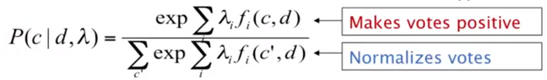
- It is a probabilistic distribution: it estimates a probability for each class/label, aka Softmax.
- It is a classifier, deciding how to weight features, given data. choose the highest probability label.
- Application: dependency parsing actions prediction, text classification, Word sense disambiguation
Training Discriminative Model
- Features in NLP are more general, they specify indicator function(a yes/no
[0,1]boolean matching function) of properties of the input and each class. - Weights: low possibility features will associate with low/negative weight, vise versa.
- Define features: Pick sets of data points d which are distinctive enough to deserve model parameters: related words, words contians #, words end with ing, etc.
Regularization in Discriminative Model
The issue of scale:
- Lots of features
- sparsity:
- easily overfitting: need smoothing
- Many features seen in training never occur again in test
- Optimization problem: feature weights can be infinite, and iterative solvers can take a long time to get to those infinities. See tutorial 4.
- Solution:
- Early stopping
- Smooth the parameter via L2 regularization.
- Smooth the data, like the add alpha smoothing, but hard to know what artificial data to create
Morphology
构词学(英语言学分科学名:morphology,“组织与形态”),又称形态学,是语言学的一个分支,研究单词(word)的内部结构和其形成方式。如英语的dog、dogs和dog-catcher有相当的关系,英语使用者能够利用他们的背景知识来判断此关系,对他们来说,dog和dogs的关系就如同cat和cats,dog和dog-catcher就如同dish和dishwasher。构词学正是研究这种单字间组成的关系,并试着整理出其组成的规则。
Morphemes: The way words are built up from smaller meaning-bearing units.
Lemma:
- Lexeme, refers to the set of all the forms that have the same meaning,
- lemma: refers to the particular form that is chosen by convention to represent the lexeme.
- E.g:
run, runs, ran, runningare forms of the same lexeme, with run as the lemma.
Affixes: Adding additional meanings of various kinds. “+ed, un+”
- suffix : follow the stem
- Plural of nouns ‘cat+s’
- Comparative and superlative of adjectives ‘small+er’
- Formation of adverbs ‘great+ly’
- Verb tenses ‘walk+ed’
- All inflectional morphology in English uses suffixes
- Prefix: precede the stem
- In English: these typically change the meaning
- Adjectives ‘un+friendly’, ‘dis+interested’
- Verbs ’re+consider’
- Some language use prefixing much more widely
- Infix: inserted inside the stem
- Circumfix: do both(follow, precede)
Root, stem and base are all terms used in the literature to designate that part of a word that remains when all affixes have been removed.
- The root word is the primary lexical unit of a word, and of a word family (this root is then called the base word), which carries the most significant aspects of semantic content and cannot be reduced into smaller constituents.
- E.g: In the form ‘untouchables’ the root is ‘touch’, to which first the suffix ‘-able’, then the prefix ‘un-‘ and finally the suffix ‘-s’ have been added. In a compound word like ‘wheelchair’ there are two roots, ‘wheel’ and ‘chair’.
Stem is of concern only when dealing with inflectional morphology
- Stemming: reduce terms to their stems in info retrieval,
- E.g: In the form ‘untouchables’ the stem is ‘untouchable’, ‘touched’ -> ‘touch’; ‘wheelchairs’ -> ‘wheelchair’.
Morphological Parsing
Use Finite-state transducers, FST, a transducer maps between one representation and another; It is a kind of FSA which maps between two sets of symbols.
Inflectional vs. Derivational Morphology
Inflectional · nouns for count (plural: +s) and for possessive case (+’s) · verbs for tense (+ed, +ing) and a special 3rd person singular present form (+s) · adjectives in comparative (+er) and superlative (+est) forms.
Derivational · Changing the part of speech, e.g. noun to verb: ‘word → wordify’ · Changing the verb back to a noun · Nominalization: formation of new nouns, often verbs or adjectives
| Inflectional | Derivational |
|---|---|
| does not change basic meaning or part of speech | may change the part of speech or meaning of a word |
| expresses grammatical features or relations between words | not driven by syntactic relations outside the word |
| applies to all words of the same part of speech, inflection occurs at word edges: govern+ment+s, centr+al+ize+d | applies closer to the stem |
Challenge of Rich Morphology
For a morphologically rich language, many issues would arise because of the morphological complexity.
- These productive word-formation processes result in a large vocabulary for these languages
- Large vocabularies mean many unknown words, and these unknown words cause significant performance degradations in a wide variety of languages
- For POS, augmentations become necessary when dealing with highly inflected or agglutinative languages with rich morphology like Czech, Hungarian and Turkish., part-of-speech taggers for morphologically rich languages need to label words with case and gender information. Tagsets for morphologically rich languages are therefore sequences of morphological tags rather than a single primitive tag.
- Dependency grammar is better than constituency in dealing with languages that are morphologically rich。
Linguistic and Representational Concepts
Parsing
- Parsing is a combination of recognizing an input string and assigning a correct linguistic structure/tree to it based on a grammar.
- The Syntactic, Statistical parsing are constituent-based representations(context-free grammars).
- The Dependency Parsing are based on dependency structure(dependency grammars).
Syntactic Parsing
Syntactic parsing, is the task of recognizing a sentence and assigning a correct syntactic structure to it.
- Syntactic parsing can be viewed as a search
- search space: all possible trees generated by the grammar
- search guided by the structure of the space and the input.
- search direction
- top-down: start with root category (S), choose expansions, build down to words.
- bottom-up: build subtrees over words, build up to S.
- Search algorithm/strategy: DFS, BFS, Recursive descent parsing, CKY Parsing
- Challenge: Structual Ambiguity
Statistical Parsing
Or probabilistic parsing, Build probabilistic models of syntactic knowledge and use some of this probabilistic knowledge to build efficient probabilistic parsers.
- motivation: to solve the problem of disambiguation
- algorithm: probability CKY parsing
- evaluation: Compare the output constituency parser with golden standard tree, a constituent(part of the output parser) marked as correct if it spans the same sentence positions with the corresponding constituent in golder standard tree. Then we get the precision, recall and F1 measure.
- constituency: S-(0:10), NP-(0:2), VP-(0:9)…
- Precission = (# correct constituents)/(# in parser output), recall = (# correct constituents)/(# in gold standard)
- Not a good evaluation, because it higher order constituent is marked wrong simply it contains a lower level wrong constituent.
Dependency Parsing
Constituency
Dependency
Morphology
Ambiguity
- Structural ambiguity: Occurs when the grammar can assign more than one parse to a sentence.
- Attachment ambiguity: A sentence has an attachment ambiguity if a particular constituent can be attached to the parse tree at more than one place.
- Coordination ambiguity: different sets of phrases can be conjoined by a conjunction like and. E.g
green egg and bread.- Coordination: The major phrase types discussed here can be conjoined with conjunctions like
and, or, and butto form larger constructions of the same type.
- Coordination: The major phrase types discussed here can be conjoined with conjunctions like
- Global and local ambiguity
- global ambiguity: multiple analyses for a full sentence, like
I saw the man with the telescope - local ambiguity: multiple analyses for parts of sentence.
the dog bit the child: first three words could be NP (but aren’t).- Building useless partial structures wastes time.
- global ambiguity: multiple analyses for a full sentence, like
Open-class Closed-class
Closed classes are those with relatively fixed membership
- prepositions: on, under, over, near, by, at, from, to, with
- determiners: a, an, the
- pronouns: she, who, I, others
- conjunctions: and, but, or, as, if, when
- auxiliary verbs: can, may, should, are
- particles: up, down, on, off, in, out, at, by
- numerals: one, two, three, first, second, third
Open-class
- Nouns, verbs, adjectives, adverbs
Word Sense
A discrete representation of an aspect of a word’s meaning. How: Distributional semantic models
Collocation: A sequence of words or terms that co-occur more often than would be expected by chance.
Synonym: 代名词, When two senses of two different words (lemmas) are identical, or nearly identical, the two senses are synonyms. E.g. couch/sofa vomit/throw up filbert/hazelnut car/automobile
Similarity: Or distance, a looser metric than synonymy. Two ways to measure similarity:
- Thesaurus词库-based: are words nearby in hypernym hierarchy? Do words have similar definitions?
- Distributional: do words have similar distributional contexts
Hyponym: 下义词, One sense is a hyponym of another sense if the first sense is more specific, denoting a subclass of the other. E.g. car is a hyponym of vehicle; dog is a hyponym of animal, and mango is a hyponym of fruit.
Hypernym: Superordinate, 上位词, vehicle is a hypernym of car, and animal is a hypernym of dog.
Word Sense Disambiguation
WSD, The task of selecting the correct sense for a word, formulated as a classification task.
- Chose features: Directly neighboring words, content words, syntactically related words, topic of the text, part-of-speech tag, surrounding part-of-speech tags, etc …
Distributional Semantic Models
Vector semantics(embeddings): The meaning of a word is represented as a vector.
- Two words are similar if they have similar word contexts vector.
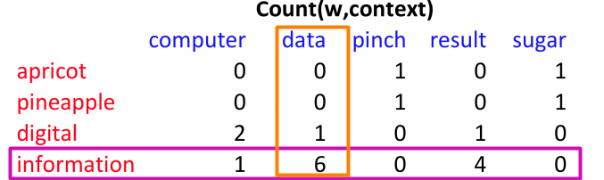
- Term-context matrix(Co-occurrence Matrices): a word/term is defined by a vector over counts of context words. The row represent words, columns contexts.
- Problem: simple frequency isn’t the best measure of association between words. One problem is that raw frequency is very skewed and not very discriminative. “the” and “of” are very frequent, but maybe not the most discriminative.
- Sulution: use Pointwise mutual information. Then the Co-occurrence Matrices is filled with PPMI, instead of raw counts.
- Measuring vectors similarity based on PPMI:
- Dot product(inner product): More frequent words will have higher dot products, which cause similarity sensitive to word frequency.
- Cosine: normalized dot product
 , Raw frequency or PPMI is non-negative, so cosine range
 [0,1].
- Evaluation of similarity
- Intrinsic: correlation between algorithm and human word similarity ratings.
- Check if there is correlation between similarity measures and word frequency.
- Application: sentiment analysis, see lab8
Pointwise Mutual Information
PMI: do events x and y co-occur more than if they were independent?
- PMI between two words: $$PMI(w, c) = \log_2 \frac{P(w,c)}{P(W)P(c)}$$
- Compute PMI on a term-context matrix(using counts): $$PMI(x, y) = log_2 \frac{N \times count(x, y)}{Count(x) Count(y)}$$
p(w=information, c=data) = 6/19
p(w=information) = 11/19
p(c=data) = 7/19
PMI(information,data) = log2(6*19/(11*7))
- PMI is biased towards infrequent events, solution:
- Add-one smoothing
PPMI: Positive PMI, could better handle low frequencies
PPMI = max(PMI,0)
T-test
The t-test statistic, like PMI, can be used to measure how much more frequent the association is than chance.
- The t-test statistic computes the difference between observed and expected means, normalized by the variance.
- The higher the value of t, the greater the likelihood that we can reject the null hypothesis.
- Null hypothesis: the two words are independent, and hence P(a,b) = P(a)P(b) correctly models the relationship between the two words.$$t\textrm{-}test(a,b) = \frac{P(a,b) - P(a)P(b)}{\sqrt{P(a)P(b)}}$$
Minimum Edit Distance
the minimum number of editing operations (operations like insertion, deletion, substitution) needed to transform one string into another. Algorithm: searching the shortest path, use Dynamic programming to avoid repeating, (use BFS to search the shortest path?)
WordNet
A hierarchically organizesd lexical database, resource for English sense relations
- Synset: The set of near-synonyms for a WordNet sense (for synonym set)
Word2Vec
Sentence Meaning Representation
我们假设语言表达具有意义表征,这些表征由用于表示常识的类型相同的东西组成。而创建这种表征并将其分配给输入的语言的任务,称为语义分析(Semantic Analysis)。The symbols in our meaning representations language (MRL) correspond to objects, properties, and relations in the world.  上图展示了使用四种常用的MRL表达“I have a car”,第一行是First order logic,有向图和其文字信息是 Abstract Meaning Representation (AMR),其余两种是Frame-Based 和 Slot-Filler。
Qualifications of MRL:
- Canonical form: sentences with the same (literal) meaning should have the same MR.
- Compositional: The meaning of a complex expression is a function of the meaning of its parts and of the rules by which they are combined.
- Verifiable: Can use the MR of a sentence to determine the truth of the sentence with respect to some given model(knowledge base) of the world.
- Unambiguous: an MR should have exactly one interpretation.
- Inference and Variables: we should be able to verify sentences not only directly, but also by drawing conclusions based on the input MR and facts in the knowledge base.
- Expressiveness: the MRL should allow us to handle a wide range of meanings and express appropriate relationships between the words in a sentence.
Lexical semantics: the meaning of individual words.
Lexical semantic relationships: Relations between word senses
模型论
从仅是正式的陈述到能够告诉我们世界某些事态的陈述,我们期望 meaning representations 弥合这种差距。而提供这种保证的依据就是模型。模型是一种正式的结构,可以代表真是世界的特定事态。
意义表达的词汇表包含两部分:
- 非逻辑词汇表,由构成我们试图表达的世界的对象,属性和关系的开放式名称组成。如 谓语predicates, nodes, labels on links, or labels in slots in frames。
- 逻辑词汇表,由一组封闭的符号,运算符,量词,链接等组成,它们提供了用给定意义表示语言编写表达式的形式化方法。
所有非逻辑词汇的元素都需要在模型中有一个表示(属于模型的固定的且定义明确的一部分)。 • 对象 Objects denote elements of the domain • 属性 Properties denote sets of elements of the domain • 关系 Relations denote sets of **tuples of elements of the domain
First-order Logic
FOL, Predicate logic, meets all of the MRL qualifications except compositionality.
- Term: represent objects.
- Expressions are constructed from terms in three ways:
- Constants in FOL refer to specific objects in the world being described. FOL constants refer to exactly one object. Objects can, however, have multiple constants that refer to them.
- Functions in FOL correspond to concepts that are often expressed in English as genitives(所有格) 如 “Frasca’s location”, 一般表达为
LocationOf(Frasca). Functions provide a convenient way to refer to specific objects without having to associate a named constant with them. - Variables, 允许我们对对象做出断言和推理,而不必引用任何特定的命名对象。Make statements about anonymous objects: making statements about a particular unknown object and making statements about all the objects in some arbitrary world of objects.
Predicate(谓语, 谓词, 宾词, 述语): symbols that represent properties of entities and relations between entities.
- Terms can be combined into predicate-argument structures.
Restaurant(Maharani)指明Maharani的属性是Restaurant. - Predicates with multiple arguments represent relations between entities:
member-of(UK, EU) /Nto indicate that a predicate takes N arguments:member-of/2
Logical connectives: create larger representations by conjoining logical formulas using one of three operators. ∨(or), ∧(and), ¬(not), ⇒(implies). “I only have five dollars and I don’t have a lot of time.”, Have(Speaker,FiveDollars) ∧ ¬Have(Speaker,LotOfTime)
Variables and Quantifiers:
- Existential Quantifiers: (“there exists”), “a restaurant that serves Mexican food near ICSI” -
∃xRestaurant(x) ∧ Serves(x, MexicanFood) ∧ Near((LocationOf(x), LocationOf(ICSI)), 头部的∃告诉我们如何解读句中的变量x: 要让句子为真, 那么对于变量x至少存在一个对象。 - Universal Quantifier:
∀(“for all”). “All vegetarian restaurants serve vegetarian food.” -∀xVegetarianRestaurant(x) ⇒ Serves(x,VegetarianFood).
A predicate with a variable among its arguments only has a truth value if it is bound by a quantifier: ∀x.likes(x, Gim) has an interpretation as either true or false.
Lambda Notation
Extend FOL, to work with ‘partially constructed’ formula, with this form λx.P(x).
λ-reduction: 应用于逻辑 term 以产生新的FOL表达式, 其中形参变量绑定到指定的term, 形式为λx.P(x)(A) -> P(A). E.g.:λx.sleep(x)(Marie) -> sleep(Marie)
- 嵌套使用, Verbal (event) MRs:
λx.λy.Near(x,y)(Bacaro)->λy.Near(Bacaro,y),λz. λy. λx. Giving1(x,y,z) (book)(Mary)(John)->Giving1(John, Mary, book)->John gave Mary a book - Problem:
- fixed arguments
- Requires separate
Givingpredicate for each syntactic subcategorisation frame(number/type/position of arguments). - Separate predicates have no logical relation: if
Giving3(a, b, c, d, e)is true, what aboutGiving2(a, b, c, d)andGiving1(a, b, c).
- Solution: Reification of events 事件具象化
Inference
推断的两种思路, forward chaining 和 backward chaining.
forward chaining systems:
Modus ponens(if - then) states that if the left-hand side(antecedent) of an implication rule is true, then the right-hand side(consequent) of the rule can be inferred.
VegetarianRestaurant(Leaf)
∀xVegetarianRestaurant(x) ⇒ Serves(x,VegetarianFood)
then
Serves(Leaf ,VegetarianFood)
随着单个事实被添加到知识库中,modus ponens用于触发所有适用的implication rules。优点是事实可以在被在需要时才在知识库中呈现,因为在某种意义上来说所有推断都是预先执行的。这可以大大减少后续的queries所需的时间,因为都应该是简单的查找。但缺点是那些永远用不到的事实也可能被推断和存储。
backward chaining:
- 第一步是通过查看query公式是否存在知识库中, 来确认query是否为真。比如查询
Serves(Leaf ,VegetarianFood). - 如果没有,则搜索知识库中存在的适用implication rules。对涉及到的antecedent递归运行backward chaining. 比如发动搜索适用规则,从而找到规则
∀xVegetarianRestaurant(x) ⇒ Serves(x,VegetarianFood), 对于termLeaf而言, 对应的antecedent是VegetarianRestaurant(Leaf), 存在于知识库中.
Prolog 就是采用backward chaining 推断策略的编程语言.
虽然forward和backward推理是合理的,但两者都不完备。这意味着单独使用这些方法的系统无法找到有效的推论。完备的推理是解析 resolution, 但计算成本很高. 在实践中,大多数系统使用某种形式的chaining并把负担压到知识库开发人员去解码知识,以支持必要inference可以推论.
Reification of Events
John gave Mary a book -> ∃e, z. Giving(e) ∧ Giver(e, John) ∧ Givee(e, Mary) ∧ Given(e,z) ∧ Book(z)
- Reify: to “make real” or concrete, i.e., give events the same status as entities.
- In practice, introduce variables for events, which we can quantify over
- Entailment relations: automatically gives us logical entailment relations between events
[John gave Mary a book on Tuesday] -> [John gave Mary a book]
∃ e, z. Giving(e) ∧ Giver(e, John) ∧ Givee(e, Mary) ∧ Given(e,z) ∧ Book(z) ∧ Time(e, Tuesday)
->
∃ e, z. Giving(e) ∧ Giver(e, John) ∧ Givee(e, Mary) ∧ Given(e,z) ∧ Book(z)
Semantic Parsing
Aka semantic analysis. Systems for mapping from a text string to any logical form.
- Motivation: deriving a meaning representation from a sentence.
- Application: question answering
- Method: Syntax driven semantic analysis with semantic attachments
Syntax Driven Semantic Analysis
- Principle of compositionality: the construction of constituent meaning is derived from/composed of the meaning of the constituents/words within that constituent, guided by word order and syntactic relations.
- Build up the MR by augmenting CFG rules with semantic composition rules. Add semantic attachments to CFG rules.
- Problem: encounter invalide FOL for some (base-form) MR, need type-raise.
- Training
Semantic Attachments
E.g
VP → Verb NP : {Verb.sem(NP.sem)}
Verb.sem = λy. λx. ∃e. Serving(e) ∧ Server(e, x) ∧ Served(e, y)
NP.sem = Meat
->
VP.sem = λy. λx. ∃e. Serving(e) ∧ Server(e, x) ∧ Served(e, y) (Meat)
= λx. ∃e. Serving(e) ∧ Server(e, x) ∧ Served(e, Meat)
The MR for VP, is computed by applying the MR function to VP’s children.
Complete the rule:
S → NP VP : {VP.sem(NP.sem)}
VP.sem = λx. ∃e. Serving(e) ∧ Server(e, x) ∧ Served(e, Meat)
NP.sem = AyCaramba
->
S.sem = λx. ∃e. Serving(e) ∧ Server(e, x) ∧ Served(e, Meat) (AyCa.)
= ∃e. Serving(e) ∧ Server(e, AyCaramba) ∧ Served(e, Meat)
Abstract Meaning Representation
AMR是Rooted,带标签的digraph,易于人们阅读,易于程序处理。扩展了PropBank的Frames集合。AMR 的特点是将句子中的词抽象为概念,因而使最终的语义表达式与原始的句子没有直接的对应关系,对相同意思的不同句子能够抽象出相同的表达。
Knowledge-driven AMRL
- The Alexa Meaning Representation Language
- World Knowledge for Abstract Meaning Representation Parsing:依赖于wordnet,而中文本身就是字组词,
- Knowledge-driven Abstract Meaning Representation
AMR is bias towards English.
Slot-fillers/Template-filling/Frame
在文档中找到此类情况并填写模板位置。这些空位填充符可以包含直接从文本中提取的文本段,也可以包括通过额外处理从文本元素中推断出的诸如时间,数量或本体实体之类的概念
许多文本包含事件的报告,以及可能的事件序列,这些报告通常对应于世界上相当普遍的刻板印象。这些抽象的情况或story,和 script(Schank and Abelson,1975)有关,由子事件,参与者及其角色的原型序列组成。类似的定义还有 Frame ( Minsky(1974),Hymes(1974)和Goffman(1974)大约在同一时间提出的一系列相关概念) 和 schemata(Bobrow and Norman,1975)。
Topic Modelling
假如知道有什么主题,或者对主题的数量和分布做出先验假设,此时可以使用监督学习, 如朴素贝叶斯分类, 把文章处理成词袋(bag of words). 但假如不知道这些先验呢?
就要依靠无监督学习, 比如聚类:Instead of using supervised topic classification – rather not fix topics in advance nor do manual annotation, Use clustering to teases out the topics. Only the number of topics is specified in advance.
这就是主题建模(Topic Modelling), 一种常用的文本挖掘方法,用于发现文本中的隐藏语义结构。此时主题数量就是一个超参数, 通过主题建模,构建了单词的clusters而不是文本的clusters。因此,文本被表达为多个主题的混合,每个主题都有一定的权重。
因为主题建模不再是用词频来表达, 而是用主题权重{Topic_i: weight(Topic_i, T) for Topic_i in Topics}, 所以主题建模也是一种 Dimensionality Reduction.
主题建模也可以理解为文本主题的tagging任务, 只是无监督罢了.
主题建模的算法:
- (p)LSA: (Probabilistic) Latent Semantic Analysis – Uses Singular Value Decomposition (SVD) on the Document-Term Matrix. Based on Linear Algebra. SVD假设了Gaussian distributed.
- LDA: latent Dirichlet allocation, 假设了multimonial distribution。
LDA
LDA是pLSA的generalization, LDA的hyperparameter设为特定值的时候,就specialize成 pLSA 了。从工程应用价值的角度看,这个数学方法的generalization,允许我们用一个训练好的模型解释任何一段文本中的语义。而pLSA只能理解训练文本中的语义。(虽然也有ad hoc的方法让pLSA理解新文本的语义,但是大都效率低,并且并不符合pLSA的数学定义。)这就让继续研究pLSA价值不明显了。
- Latent Dirichlet allocation(LDA): each document may be viewed as a mixture of various topics where each document is generated by LDA.
- A topic is a distribution over words
- generate document:
- Randomly choose a distribution over topics
- For each word in the document
- randomly choose a topic from the distribution over topics
- randomly choose a word from the corresponding topic (distribution over the vocabulary)
- training: repeat until converge
- assign each word in each document to one of T topics.
- For each document d, go through each word w in d and for each topic t, compute: p(t|d), P(w|t)
- Reassign w to a new topic, where we choose topic t with probability P(w|t)xP(t|d)
- Inference: LDA没法做精确inference,只有近似算法,比如variational inference。
Evaluation
Extrinsic Evaluation
Use something external to measure the model. End-to-end evaluation, the best way to evaluate the performance of a language model is to embed it in an application and measure how much the application improves.
- Put each model in a task: spelling corrector, speech recognizer, MT system
- Run the task, get an accuracy for A and for B
- How many misspelled words corrected properly
- How many words translated correctly
- Compare accuracy for A and B
Unfortunately, running big NLP systems end-to-end is often very expensive.
Intrinsic Evaluation
Measures independenly to any application. Train the parameters of both models on the training set, and then compare how well the two trained models fit the test set. Which means whichever model assigns a higher probability to the test set
Human Evaluation
E.g to know whether the email is actually spam or not, i.e. the human-defined labels for each document that we are trying to gold labels match. We will refer to these human labels as the gold labels.
Precision, Recall, F-measure
- To deal with unbalanced lables
- Application: text classification, parsing.
- Evaluation in text classification: the 2 by 2 contingency table
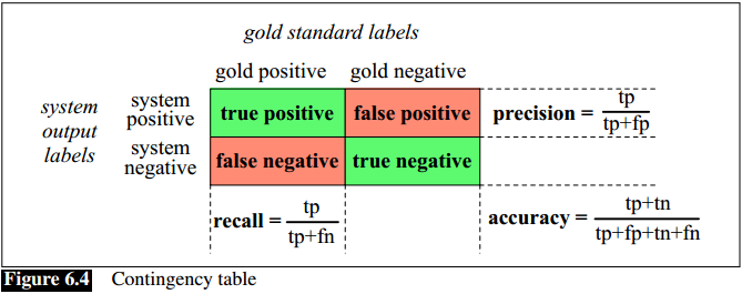 , golden lable is true or false, the classifier output is positive or negative.
Precision: Percentage of positive items that are golden correct, from the view of classifier
Recall: Percentage of golden correct items that are positive, from the view of test set.
F-measure
- Motivation: there is tradeoff between precision and recall, so we need a combined meeasure that assesses the P/R tradeoff.
- The b parameter differentially weights the importance of recall and precision, based perhaps on the needs of an application. Values of b > 1 favor recall, while values of b < 1 favor precision.
- Balanced F1 measure with beta =1, F = 2PR/(P+R)
Confusion Matrix
Recalled that confusion matrix’s row represent golden label, column represent the classifier’s output, to anwser the quesion:for any pair of classes(c1,c2), how many test sample from c1 were incorrectly assigned to c2
- Recall: Fraction of samples in $c_1$ classified correctly, $\frac{CM(c_1, c_1)}{\sum_jCM(c_1, j)}$
- Precision: fraction of samples assigned $c_1$ that are actually $c_1$, $\frac{CM(c_1, c_1)}{\sum_iCM(i, c_1)}$
- Accuracy: $\frac{\sum diagnal}{all}$
Correlation
When two sets of data are strongly linked together we say they have a High Correlation. Correlation is Positive when the values increase together, and Correlation is Negative when one value decreases as the other increases.
- Pearson correlation: covariance of the two variables divided by the product of their standard deviations.$$r = \frac{\sum_{i=1}^n(x_i - \overrightarrow{x})(y_i - \overrightarrow{y})}{\sqrt{\sum_{i=1}^n(x_i - \overrightarrow{x})^2} \sqrt{\sum_{i=1}^n(y_i - \overrightarrow{y})^2}}$$
- Spearman correlation: the Pearson correlation between the rank values of the two variables
Basic Text Processing
Regular Expressions
NLP工作必备技能(考试不需要).
一些练习Regular Expressions的有趣网站: https://alf.nu/RegexGolf https://regexr.com/
Word Tokenization
NLP task needs to do text normalization:
- Segmenting/tokenizing words in running text
- Normalizing word formats
- Segmenting sentences in running text
they lay back on the San Francisco grass and looked at the stars and their
- Type: an element of the vocabulary.
- Token: an instance of that type in the actual text.
英文比较简单. 中文有一个难点, 需要分词.