Inf Course Note - Natural Language Understanding

爱丁堡大学信息学院课程笔记 Natural Language Understanding, Informatics, University of Edinburgh

References: Natural language understanding CS224n: Natural Language Processing with Deep Learning Lecture Slides from the Stanford Coursera course Natural Language Processing, by Dan Jurafsky and Christopher Manning

Meaning representations

意思的表达有很多方法。一种有效的表示单词的含义的方法是 distributional semantic.

Semantics (from Ancient Greek: σημαντικός sēmantikos, “significant”) is the linguistic and philosophical study of meaning, in language, programming languages, formal logics, and semiotics.

语义学 Semantics 在语言学中的研究目的在于找出语义表达的规律性、内在解释、不同语言在语义表达方面的个性以及共性；与计算机科学相关的语义学研究在于机器对自然语言的理解。

Tradition solution of usable meaning in a computer: Use e.g. WordNet, a resource containing lists of synonym sets and hypernyms.

To convert natural language into values that computer understands, represent words as discrete symbols: Words can be represented by one-hot vectors, Vector dimension is the vocabulary. But there is no natural notion of similarity for one-hot vectors!

So learn to encode similarity in the vectors themselves.

The core idea is representing words by their context, building a dense vector for each word, chosen so that it is similar to vectors of words that appear in similar contexts.

Distributional models of meaning = vector-­space models of meaning = vector semantics. word vectors = word embeddings = word representations.

Four kinds of vector models

Sparse vector representations: 1, Mutual-­information weighted word co-­occurrence matrices

Dense vector representations: 2, Singular value decomposition (SVD): A special case of this is called LSA - Latent Semantic Analysis 3, Neural­‐network­‐inspired models (skip­‐grams, CBOW) 4, Brown clusters

Prediction-­based models learn embeddings as part of the process of word prediction. Train a neural network to predict neighboring words. The advantages: · Fast, easy to train (much faster than SVD) · Available online in the word2vec package · Including sets of pretrained embeddings

Word representation and Word2vec

Word2vec is a framework for learning word vectors representation. Idea: 1, We have a large corpus of text 2, Every word in a fixed vocabulary is represented by a vector 3, Go through each position t in the text, which has a center word c and context (“outside”) words o 4, Use the similarity of the word vectors for c and o to calculate the probability of o given c (or vice versa) 5, Keep adjusting the word vectors to maximize this probability

在上面第四点, 如果是给定中心词，计算上下文词, 那么就是 Skip-grams model, 比如 Given word $w_t$, in a context window of 2C words, predict 4 context words [w_t-2, w_t-1, w_t+1, w_t+2] Skip-grams 给予模型跳词能力，比如 “I hit the tennis ball” 有三个trigrams: “I hit the”, “hit the tennis”, “the tennis ball”. 但是，这个句子也同样包含一个同样重要但是N-Gram无法提取的trigram:“hit the ball”. 而使用 skip-grams 允许我们跳过 “tennis” 生成这个trigram.

反之，给定 bag-of-words context, predict target word, 那就是 Continuous Bag of Words, CBOW model.

缺点：因为output size 等于 vocabulary，而 softmax 分母中需要求和每一个词的 output size × hidden units 的内积， 计算会非常昂贵。解决办法是使用负采样 negative sampling。

Word2vec的本质是遍历语料库的每一个词$w_i$，捕捉$w_i$与其上下文位置目标词的同时出现的概率。

目标函数

Obejective funtion (cost or loss function) J(θ): For each position $t = 1, … , T$, predict context words within a window of fixed size m, given center word, use chain rule to multiply all the probability to get the likelihood $L(θ)$: The θ is the vectors representations, which is the only parameters we needs to optimize(其实还有其他hyperparameters，这里暂时忽略).

The loss function is the (average) negative log likelihood:

Minimizing objective function ⟺ Maximizing predictive accuracy.

The problem is how to calculate $P(w_{t+j} \mid w_t; θ)$:

每个词由两个向量表示（Easier optimization. Average both at the end）： $v_w$ when w is a center word, $u_w$ when w is a context word.

Then for a center word c and a “outside” word o: The numerator contains dot product, compares similarity of o and c, larger dot product = larger probability. The denominator works as a normalization over entire vocabulary.

高频词二次采样

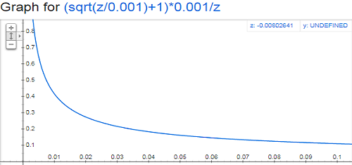
subsampling 二次采样是指当决定是否选取一个词作为样本时，它被选择的概率反比于它出现的概率，这样不仅可以降低无意义但高频的词(“the”, “a"等)的重要性，也可以加快采样速度。$$P(w_i) = (\sqrt{\frac{z(w_i)}{0.001}} + 1) \cdot \frac{0.001}{z(w_i)}$$ $z(w_i)$ 是词$w_i$在语料库中的占比，如果"peanut"在10亿语料库中出现了1,000次, 那么z(“peanut”) = 1e-6.

Negative sampling

负采样是指每个训练样本仅更新模型权重的一小部分：only the output that represents the positive class(1) + other few randomly selected classes(0) are evaluated. 该论文指出

负采样5-20个单词适用于较小的数据集，对于大型数据集只需要2-5个单词。

修改目标函数，选择k个负样本（即除了概率最高的那个目标词之外的其他词）：

这样可以最大化真正的外部词出现的概率，最小化随机负采样的词概率。

负面样本的选择是基于 unigram 分布 $f(w_i)$: 一个词作为负面样本被选择的概率与其出现的频率有关，更频繁的词更可能被选作负面样本。 $$P(w_i) = \frac{ {f(w_i)}^{3/4} }{\sum_{j=0}^{n}\left( {f(w_j)}^{3/4} \right) }$$ 负采样的优点是： · Training speed is independent of the vocabulary size · Allowing parallelism. · 模型的表现更好。因为负采样契合NLP的稀疏性质，大部分情况下，虽然语料库很大，但是每一个词只跟很小部分词由关联，大部分词之间是毫无关联的，从无关联的两个词之间也别指望能学到什么有用的信息，不如直接忽略。

与传统的NLP方法比较

在word2vec出现之前，NLP使用经典且直观的共生矩阵（co-occurrence matrix）来统计词语两两同时出现的频率，参考ANLP - Distributional semantic models。缺点也明显，词汇量的增加导致矩阵增大，需要大量内存，随之而来的分类模型出现稀疏性问题，模型不稳定。虽然可以使用SVD来降维，但是一个n×m矩阵的计算成本是O(mn²)浮点数（当n<m），还是非常大的。而且很难并入新词或新文档。

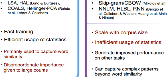
目前融合了两种方法的优点的Glove是最常用的。

TODO(Glove)

Morphological Recursive Neural Network (morphoRNN)

Limitation of word2vec: • Closed vocabulary assumption • Cannot exploit functional relationships in learning:

如英语的dog、dogs和dog-catcher有相当的关系，英语使用者能够利用他们的背景知识来判断此关系，对他们来说，dog和dogs的关系就如同cat和cats，dog和dog-catcher就如同dish和dishwasher

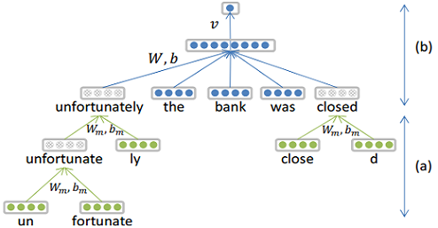
To walk closer to open vocabulary, use compositional representations based on morphemes. Instead of word embedding, embed morphemes - the smallest meaningful unit of language. Compute representation recursively from morphemes, word embedding 由 morphemes embedding 拼接而来.![](/images/Morphological_Recursive_Neural_Network.png “Morphological Recursive Neural Network. A vector representation for the word “unfortunately” is constructed from morphemic vectors: un_pre, fortunate_stm, ly_suf. Dotted nodes are computed on-the-fly and not in the lexicon. image from: http://www.aclweb.org/anthology/W13-3512")

与基础版的morphoRNN结构相同，Context-insensitive Morphological RNN model (cimRNN) 考察 morphoRNN 在不参考任何上下文信息情况下， 仅仅用 morphemic representation 构造词向量的能力。训练时，给每个词xi定义损失函数s(xi)为新构造的词向量p_c(xi)和参考词向量p_r(xi)之间的欧几里得距离平方

该cimRNN模型没有机会改进可能被估计不足的罕见词的表达.

Context-sensitive Morphological RNN (csmRNN) 在学习语素组成时同时参考语境信息，在训练过程中，神经网络顶层的更新将一直反向传播直至底层的语素层。

Compositional character representations

在自然语言处理中使用 word 作为基本单位的问题在于词汇量太大了，所以几乎所有主流模型都会省略很多词，比如Bengio的RNNs语言模型就把所有出现频率<3的单词统一标记为一个特殊词。但这样的操作也只是把词汇量降到了16,383。又比如word2vec模型只考虑出现频率最高的30,000个词。

所以寻找其他有限集合的语言单位成为替代选择，比如字母 character（更确切地说是 unicode code points），比如前面提到的 Morphemes，还有其他比如 Character n-grams，Morphological analysis等，这些可以统称为 subwords units。

然后再通过 subwords 来重构 word representation，进而构建整个文本的meaning representation.

构建 word representation 最简单的方法就是把 subwords vectors 相加、平均或者拼接等，但更好的是使用非线性的方法，比如 Bidirectional LSTMs, Convolutional NNs 等。

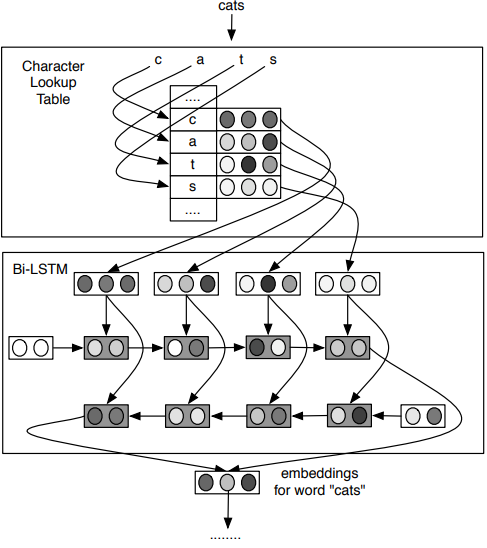
哪种方式构建 subword representations 比较好？

在 word representation 的重构中，涉及了几个变量: 1, Subword Unit

2, Composition Function • Linear Vector operation • Bi-LSTMs • Convolutional NNs

3, Language Typology

Type	example	Morphology	analysis
Fusional (English)	“reads”	read-s	read-3SG.SG
Agglutinative (Turkish)	“If I read …”	oku-r-sa-m	read-AOR.COND.1SG
Root&Pattern (Arabic)	“he wrote”	k(a)t(a)b(a)	write-PST.3SG.M
Reduplication (Indonesian)	“children”	anak~anak	child-PL

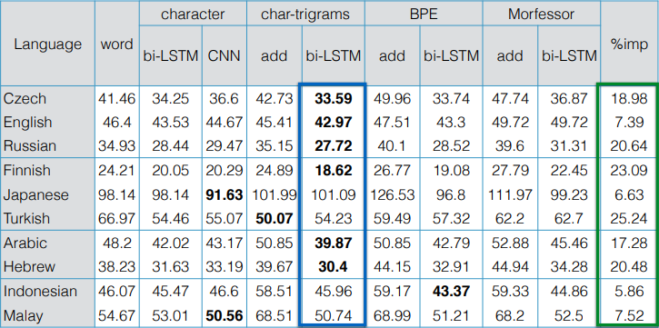
除了语言模型外, 其他NLP任务如SQuAd问答数据集上的很多优秀模型，也会加入character embedding.

但目前 Character-level models 并不具有触及实际 morphology 的模型预测能力。

Multi-word language representations

Neural bag-of-words models: · Simply average (or just sum) word vectors, · Can improve effectiveness by putting output through 1+ fully connected layers (DANs) · Recurrent neural networks(LSTM/GRU): cannot capture phrases without prefix context, and empirically, representations capture too much of last words in final vector – focus is LM next word prediction · Convolutional Neural Network: compute vectors for every h-word phrase, often for several values of h. Example: “the country of my birth” computes vectors for: the country, country of, of my, my birth, the country of, country of my, of my birth, the country of my, country of my birth. Not very linguistic, but you get everything!

Data-dependent composition: Recursion is natural for describing language, Phrases correspond to semantic units of language.

How to map longer phrases into the same vector space? 利用复合性原理 principle of compositionality:

在数学、语义学和语言哲学中，复合性原理是指，一个复杂表达式的意义是由其各组成部分的意义以及用以结合它们的规则来决定的。

Recursive neural nets, a tree structure. For Structure Prediction: Inputs: two candidate children’s representations Outputs: 1, The semantic representation if the two nodes are merged. 2, Score of how plausible the new node would be.

神经网络语言模型

如何构建一个神经网络语言模型? 语言模型的目的是输入一串字符, 输出下一个字符的概率分布, 可以使用 fixed-window neural Language Model, 类似于N-Gram, 仅考虑前(n-1)个窗口长度序列, “as the proctor started the clock the students opened their _” 得到定长的输入序列, 而 Feedforward neural networks 的输入就是要求固定长度的向量.

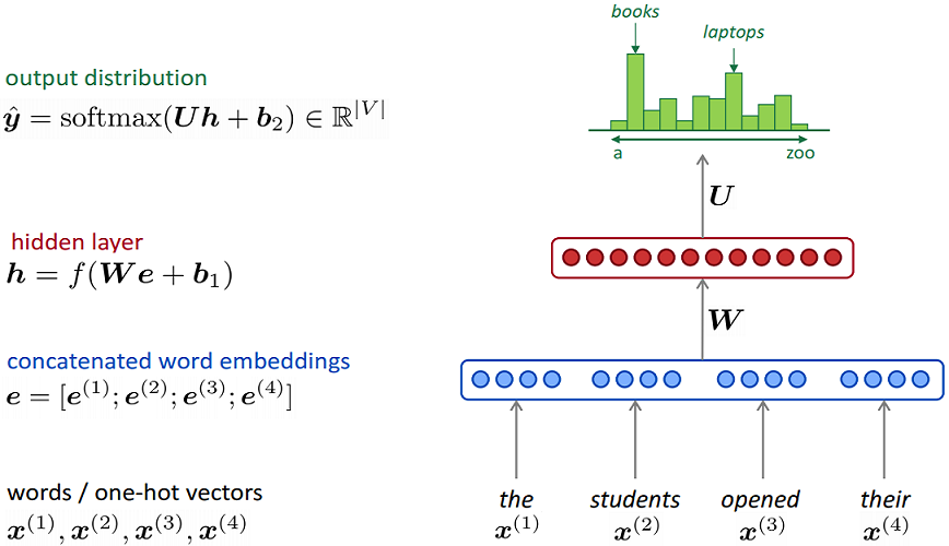
用前馈神经网络做语言模型的优点（相对于N-Gram）就是没有了稀疏性问题，而且模型的大小也控制在 O(n)（N-Gram是O(exp(n))）

固定长度的前馈神经网络的固有缺陷就是它要求输入和输出都是固定长度的, 仅考虑前的(n-1)长度的序列, 很多时候会丢失NLP中的长距离依赖信息, 跟N-Gram的有一样的缺陷。而且实际的应用中语句的长度是不固定的，最好有一个神经网络可以接受任意长度的输入序列, 输出任意长度的序列。循环神经网络 (Recurrent neural networks, aka RNNs) 就可以解决这个问题.

循环神经网络语言模型

不同于前馈神经网络使用输入序列的每一个词单独训练一行(或一列, 取决于矩阵的设计)参数矩阵, RNNs的设计核心是用输入序列的每一个词, 反复地训练同一个参数, 即"共享参数”.

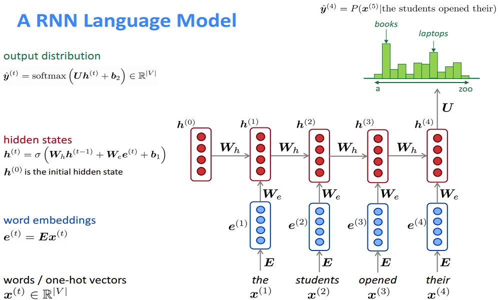
因为参数共享: 1, 模型大小不会随着输入序列长度增加而增加。 2, 每一步的计算，理论上都使用到了之前的历史信息，所以理论上可以更好的捕捉长距离依赖（但实际上表现并不好，看后面的梯度消失与爆炸）. 3, 模型有更好的泛化能力

使用基于Softmax的RNNs语言模型等同于解决矩阵分解问题, 参考Breaking the Softmax Bottleneck: A High-Rank RNN Language Model。

循环神经网络语言模型使用损失函数评估模型表现: 损失函数 loss function on step t is usual 交叉熵 cross-entropy between predicted probability distribution and the true next word.

传统的统计语言模型使用困惑度(perplexity)来评估模型表现，但其实降低困惑度等价于减小损失函数.

神经网络语言模型的学习能力

Character models are good at reduplication (no oracle, though), works well on language with reduplication patterns like Indonesian, Malay. Character NLMs learn word boundaries, memorize POS tags.

What do NLMs learn about morphology? 1, Character-level NLMs work across typologies, but especially well for agglutinative morphology. 2, predictive accuracy is not as good as model with explicit knowledge of morphology (or POS). 3, They actually learn orthographic similarity of affixes, and forget meaning of root morphemes accordong to qualitative analyses. 4, More generally, they appear to memorize frequent subpatterns

总的来说，神经网络处理自然语言的能力并不特殊，表现的性能，跟神经网络本身的长处相匹配，如泛化、模式匹配、端到端应用的能力等。

Dependency parsing

语言学里有两种角度看待语法结构 - Constituency and Dependency：

• Constituency: phrase structure grammar, 从句子成分构造的角度看，capture the configurational patterns of sentences，即把句子的语法理解为词组成分的递归嵌套. 可以用 context-free grammars (CFGs) 来表达语法规则，就是语法树。
• Dependency syntax: 主要是从语义的角度来看，显示哪些单词依赖于（一般指修改或作为参数其参数）哪些单词。特别用于区分动词的主格（subject position or with nominative inflection）宾格（object position or with accusative inflection）. Dependencies can be identified even in non-configurational languages.

A sentence dependency structure explains the dependency relation between its words: represented as a graph with the words as its nodes, linked by directed, labeled edges, with the following properties: • connected: every node is related to at least one other node, and (through transitivity) to ROOT; • single headed: every node (except ROOT) has exactly one incoming edge (from its head); • acyclic: the graph cannot contain cycles of directed edges.

Dependency trees 有两种，如果dependency graph中有edges交叉则是non-projective, 反之则是 projective。更确切的定义是：A dependency tree is projective wrt. a particular linear order of its nodes if, for all edges h → d and nodes w, w occurs between h and d in linear order only if w is dominated by h.

A non-projective dependency grammar is not context-free.

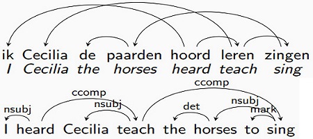
Motivation for Dependency parsing: • context-free parsing algorithms base their decisions on adjacency; • in a dependency structure, a dependent need not be adjacent to its head (even if the structure is projective); • we need new parsing algorithms to deal with non-adjacency (and with non-projectivity if present).

Evaluation: accuracy (# correct dependencies with or ignore label)).

Graph-based dependency parsing

Based on maximum spanning trees (MST parser), views syntactic structure as a set of constraints

Intuition as tagging problem: since each word has exactly one parent, the possible tags are the other words in the sentence (or a dummy node called root). If we edge factorize the score of a tree so that it is simply the product of its edge scores, then we can simply select the best incoming edge for each word.

The tartget function is to find the highest scoring dependency tree in the space of all possible trees for a sentence. The score of dependency tree y for sentence x is: $$s(x,y) = \sum_{(i,j)\in y} s(i,j)$$ $x = x_1…x_n, y$ is a set of dependency edges, with $(i, j) ∈ y$ if there is an edge from $x_i$ to $x_j$.

Scoring edges with a neural network The function g(a_j, a_i) computes an association score telling us how much word wi prefers word wj as its head. Association scores are a useful way to select from a dynamic group of candidates, 跟注意力机制的similarity score 异曲同工，方程的形式也很相似。

Parsing 算法：

• start with a totally connected graph G, i.e., assume a directed edge between every pair of words;
• find the maximum spanning tree (MST) of G, i.e., the directed tree with the highest overall score that includes all nodes of G;
• this is possible in O(n²) time using the Chu-Liu-Edmonds algorithm; it finds a MST which is not guaranteed to be projective; 1, Each node j in the graph greedily selects the incoming edge with the highest score s(i,j) 2, If result were a tree, it would have to be the maximum spanning tree; If not, there must be a cycle. 3, Break the cycle by replacing a single incoming edge to one of the nodes in the cycle. To choose the node, decide recursively by identifying the cycle and contract it into a single node and recalculate scores of incoming and outgoing edges. Now call CLE recursively on the contracted graph. MST on the contracted graph is equivalent to MST on the original graph. 这里是指先识别出循环体saw ⇄ john②，然后在这个循环体范围内，使用CLE找出 root 进出这个循环体的最大概率路线(root → saw → john = 40) > (root → john → saw = 29)③； 4, Greedily collect incoming edges to all nodes, find out to be a tree and thus the MST of the graph. 把循环体以及其包含的nodes合并为一个node wjs，并且已经有了进出wjs的最大概率路径，这样就可以在整个图上继续运行CLE算法找出最大概率路线(root → wjs → mary = 70) > (root → mary → wjs = 40)④.

Chu-Liu-Edmonds (CLE) Algorithm:

In graph theory, Edmonds’ algorithm or Chu–Liu/Edmonds’ algorithm is an algorithm for finding a spanning arborescence of minimum weight (sometimes called an optimum branching). It is the directed analog of the minimum spanning tree problem

Transition-based dependency parsing

An extension of shift-reduce parsing (MALT parser), views syntactic structure as the actions of an automaton: • for a given parse state, the transition system defines a set of actions T which the parser can take; • if more than one action is applicable, a machine learning classifier is used to decide which action to take; • just like in the MST model, this requires a mechanism to compute scores over a set of (possibly dynamic) candidates. 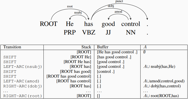if si is the ith top element on stack, and bi the ith element on buffer, then we have the following transitions: • LEFT-ARC(l): adds arc s1 → s2 with label l and removes s2 from stack (|s| ≥ 2); • RIGHT-ARC(l): adds arc s2 → s1 with label l and removes s1 from stack (|s| ≥ 2); • SHIFT: moves b1 from buffer to stack; recondition: |b| ≥ 1. 总的来说就是：父节点保留在stack中; 从始至终 root 一直都是父节点；从 buffer 中把候选词一个一个 push 到stack中，根据 classifier 预测的结果，分辨出哪个候选词是子节点，并把子节点 pop 出 stack；直到清空 buffer，stack 中只剩下 root。

Comparing MST and transition-based parsers:

Both require dynamic classifiers, and these can be implemented using neural networks, conditioned on bidirectional RNN encodings of the sentence.

The MST parser selects the globally optimal tree, given a set of edges with scores; • it can naturally handle projective and non-projective trees;

A transition-based parser makes a sequence of local decisions about the best parse action; • it can be extended to projective dependency trees by changing the transition set;

Accuracies are similar, but transition-based is faster;

Recurrent neural network grammars (RNNGs)

Widespread phenomenon: Polarity items can only appear in certain contexts, e.g. “anybody”.

In linguistics, a polarity item is a lexical item that can appear only in environments associated with a particular grammatical polarity – affirmative or negative. A polarity item that appears in affirmative (positive) contexts is called a positive polarity item (PPI), and one that appears in negative contexts is a negative polarity item (NPI).

The environment in which a polarity item is permitted to appear is called a “licensing context”.

The lecture that I gave did not appeal to anybody; The lecture that I gave appealed to anybody.

也许"anybody"出现的条件是前面出现过"not”，那么应该可以使用 RNNs 模型来解码这点信息。然而: The lecture that I did not give appealed to anybody.

这说明 Language is hierarchical: The licensing context depends on recursive structure (syntax)。不能简单根据"not"是否出现来判断，而是需要看"not"修饰的成分，也就是说要考虑语法的合理。这就给文本生成任务（或者说构建语言模型）带来挑战。

Recurrent neural network grammars (Dyer et al. 2016)提出了一种具有明确短语结构的语言模型 RNNGs。

RNNGs operate via a recursive syntactic process reminiscent of probabilistic context-free grammar generation, but decisions are parameterized using RNNs that condition on the entire syntactic derivation history, greatly relaxing context-free independence assumptions.

就是在使用 RNNs 构建语言模型，除了考虑历史词信息, 还会生成历史的语法结构, 并以此为参考预测语法结构和词语,以保证生成的语言符合语法结构。这里的语法是针对 phrase structure (constituency) grammars，所以 RNNGs 也是一种 constituency parsing：

• Generate symbols sequentially using an RNN
• Add some “control symbols” to rewrite the history periodically
  • Periodically “compress” a sequence into a single “constituent”
  • Augment RNN with an operation to compress recent history into a single vector (-> “reduce”)
  • RNN predicts next symbol based on the history of compressed elements and non-compressed terminals (“shift” or “generate”)
  • RNN must also predict “control symbols” that decide how big constituents are

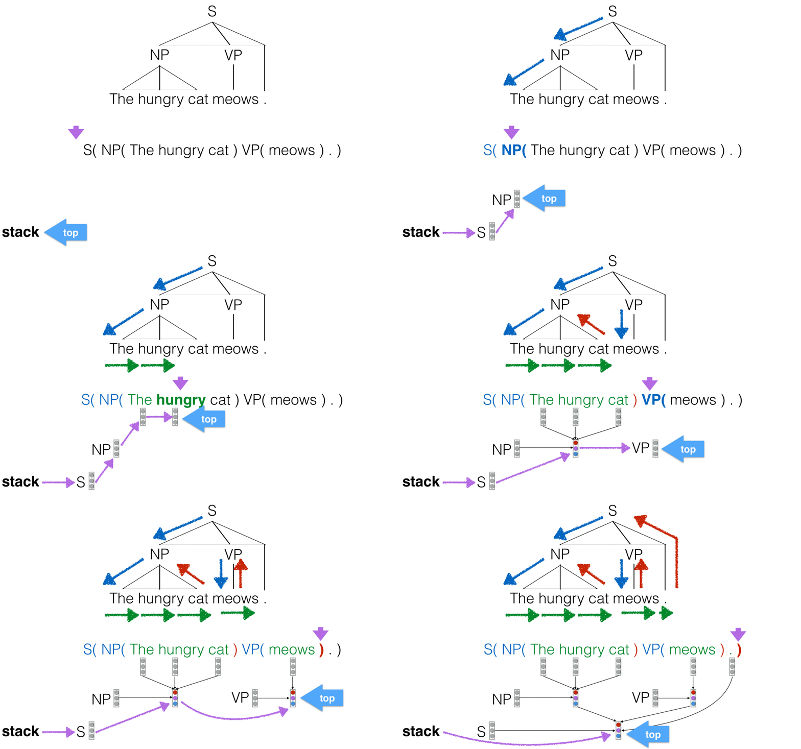
首先注意到，如果有序地去遍历语法树，得出的就是一个序列：

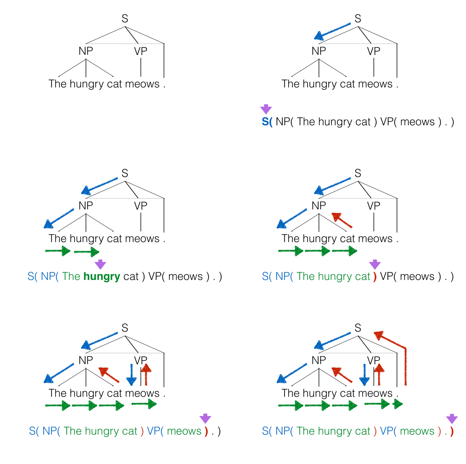
What information can we use to predict the next action, and how can we encode it with an RNN?

Use an RNN for each of:

• Previous terminal symbols
• Previous actions
• Current stack contents 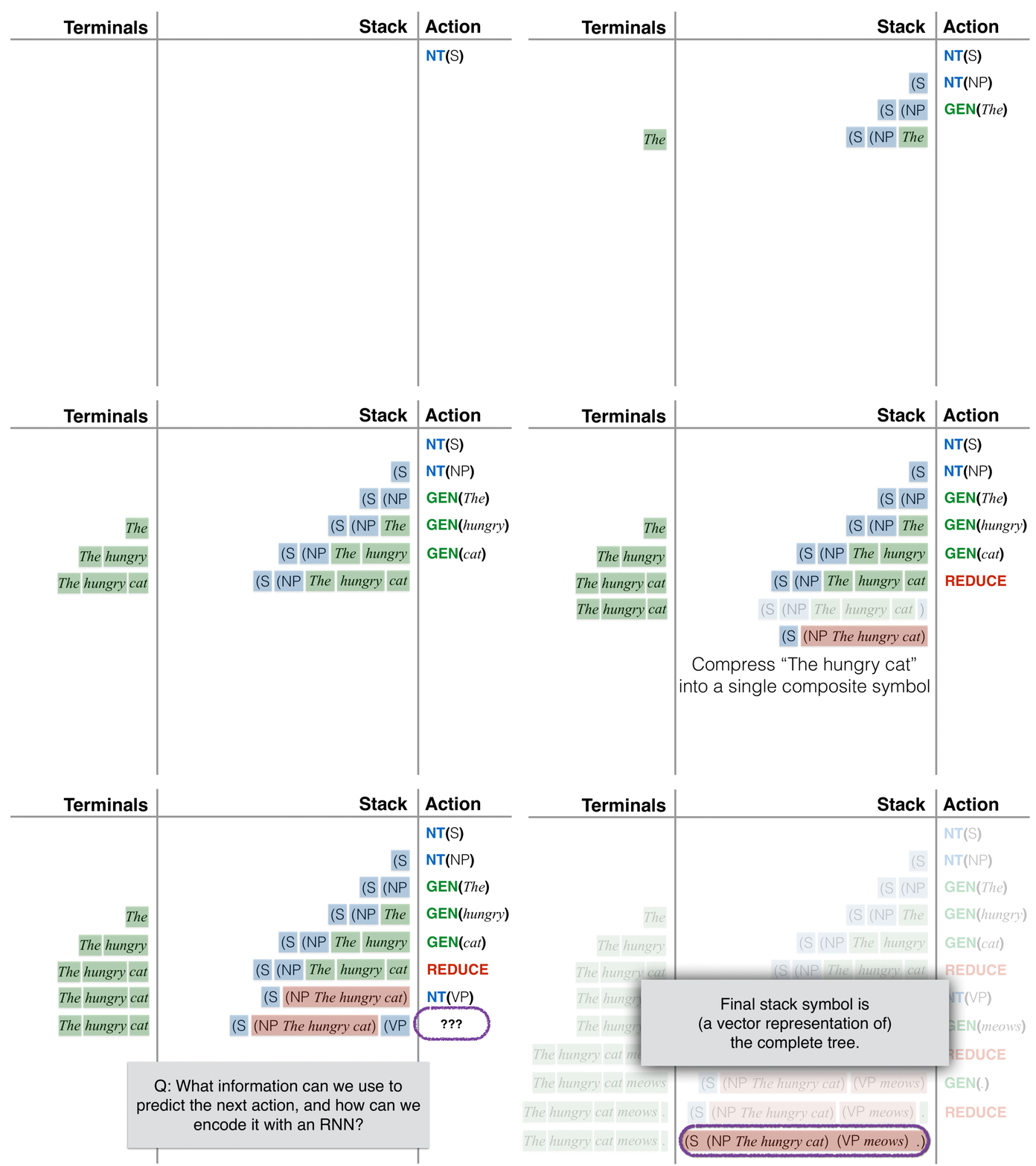最后得出的 stack 就是完整的语法树（以序列的形式）。

Syntactic Composition

人们通过较小元素的语义组合来解释较大文本单元的含义 - 实体，描述性词语，事实，论据，故事. When compressing “The hungry cat” into a single composite symbol, use Bi-LSTM to encode (NP The hungry cat).

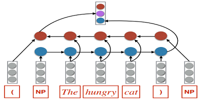
基于此可以递归地解码更复杂的短语，比如(NP The (ADJP very hungry) cat), 只需要把原来的hungry替换为(ADJP very hungry)即可。

这种递归地堆栈符号的构建行为映射了符号对应的树结构

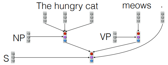
除此了使用 Bi-LSTM 解码，还可以使用 Attention：Replace composition with one that computes attention over objects in the composed sequence, using embedding of NT for similarity.

Implement RNNGs

Stack RNNs

• Augment a sequential RNN with a stack pointer
• Two constant-time operations
  • push - read input, add to top of stack, connect to current location of the stack pointer
  • pop - move stack pointer to its parent
• A summary of stack contents is obtained by accessing the output of the RNN at location of the stack pointer

Training RNNs:

• Each word is conditioned on history represented by a trio of RNNs
• backpropagate through these three RNNs, and recursively through the phrase structure S → NP VP.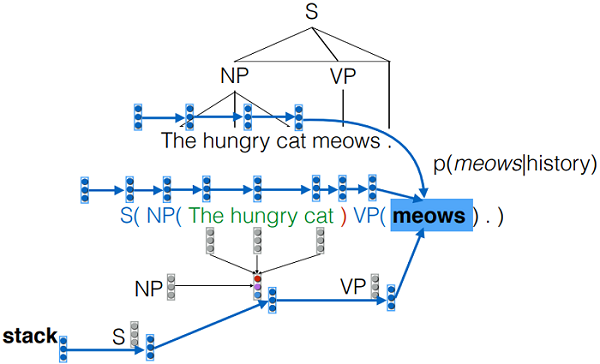

完整的RNNGs模型，用 softmax 计算下一个 action 的概率分布：

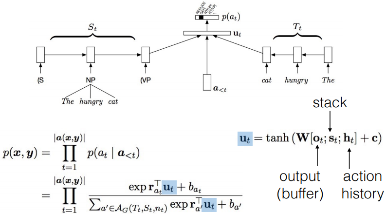
Parameter Estimation

RNNGs jointly model sequences of words together with a “tree structure”.

Any parse tree can be converted to a sequence of actions (depth first traversal) and vice versa (subject to wellformedness constraints).

Inference problems of RNNGs

An RNNG is a joint distribution p(x,y) over strings (x) and parse trees (y), i.e. it jointly predicts the word, and the parse context together. So the model will still generate the syntactic information and the next word but we can discard the additional outputs if all we want is the language model.

Two inference questions: • What is $p(x)$ for a given x? - language modeling • What is $argmax_yp(y | x)$ for a given x? - parsing

The model predicts the next action (NT() GEN() or REDUCE in generative mode, NT() SHIFT or REDUCE in discriminative mode). The set of actions completely determines the string and tree structure, so we can get their joint probability by multiplying over the probabilities of all actions.

In discriminative mode, the input is a string of words, and the model cannot generate words, but instead “consumes” the words in the input buffer. The model can be used as a parser (find the maximum prob. tree, i.e., $argmax_yP(y \mid x)$).

In generative mode, there is a respective GEN() action for every word, so the word is predicted with the action. To be a language model (find the maximum prob. sentence/assign probabilities to a sentence, i.e., $p(x)$), we must marginalize over trees to get the probability of the sentence. This is intractable so is approximated with importance sampling by sampling from a discriminatively trained model.

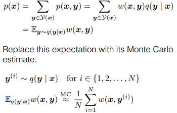
importance sampling

Assume we"ve got a conditional distribution $q(y | x)$ s.t. (i) $p(x, y) > 0 \Rightarrow q(y | x) > 0$ (ii) $y \sim q(y | x)$ is tractable and (iii) $q(y | x)$ is tractable

The importance weights $w(x,y) = \frac{p(x, y)}{q(y | x)}$

从句子到语法树的seq2seq模型

其实从句子到语法的映射类似于一个seq2seq模型。而直接的把语法树以字符序列的形式表达，使用简单的 RNNs 直接构建句子到语法序列的 seq2seq 模型效果也不错，比如： input: The hungry cat meows . output: S( NP( _ _ _ ) VP( _ ) _ ) Vanilla RNNs 在模式匹配和计数方面非常出色，经验证明，训练有素的 seq2seq 模型通常会输出格式良好的字符串，见这篇文章 section 3.2

但潜在的问题是，seq2seq 模型并不要求输出是有正确括号字符（数量对齐，位置正确）。另外，理论上单个RNN也只能记忆括号结构一定的有限深度，因为 RNNs 只有固定的有限数量的隐藏单元。例如，它将为这些输出分配非零概率： S( NP( _ _ ) VP ( _ ) _ ) S( NP( _ _ _ ) VP ( _ ) _ ) ) )

理想情况下，模型应该给任何不完整的输出分配零概率。使用 RNNGs 是因为它本身能够履行这些限制， 保证生成完整正确的语法树。

从中可以看出，seq2seq模型可以用于快速原型和 baseline 搭建，但如果遇到要求输出遵守某些约束条件的问题，则需要直接执行这些约束条件。

Parsing

Parsing is a fundamental task in NLP. But what is parsing actually good for?

Parsing breaks up sentences into meaningful parts or finds meaningful relationships, which can then feed into downstream semantic tasks: • semantic role labeling (figure out who did what do whom); • semantic parsing (turn a sentence into a logical form); • word sense disambiguation (figure out what the words in a sentence mean); • compositional semantics (compute the meaning of a sentence based on the meaning of its parts).

Semantic role labeling (SRL)

虽然可以使用 Distributional semantics 表达含义，只是 Distributional semantics 比较擅长处理相似度，且无法很明确地处理复合性 Compositionality。

在数学、语义学和语言哲学中，复合性原理是指，一个复杂表达式的意义是由其各组成部分的意义以及用以结合它们的规则来决定的。

为了能够处理复合性和推理，我们需要象征性和结构化的意义表示。

虽然语言是无穷无尽的，句子是无限的集合，而人脑的能力却是有限的，但人们总能够理解一个句子的含义（假如人们熟知表达句子的语言）. 因此, 对于 semantics, 语义肯定是有限的集合, 这样才能确定句子的确切意义.

In generative grammar, a central principle of formal semantics is that the relation between syntax and semantics is compositional.

The principle of compositionality (Fregean Principle): The meaning of a complex expression is determined by the meanings of its parts and the way they are syntactically combined.

Semantic role labeling means identifying the arguments (frame elements) that participate in a prototypical situation (frame) and labeling them with their roles;

SRL task is typically broken down into a sequence of sub-tasks:

1. parse the training corpus;
2. match frame elements to constituents;
3. extract features from the parse tree;
4. train a probabilistic model on the features.

所谓 frame elements 是针对 Frame Semantics 而言的。

SRL provides a shallow semantic analysis that can benefit various NLP applications; no parsing needed, no handcrafted features.

Frame Semantics

表达词义，除了 Firth, J.R. (1957) 的 “a word is characterized by the company it keeps”（也即是 Distributional semantics）之外, 还有 Charles J. Fillmore 的 Frame Semantics.

The basic idea is that one cannot understand the meaning of a single word without access to all the essential knowledge that relates to that word.

A semantic frame is a collection of facts that specify “characteristic features, attributes, and functions of a denotatum, and its characteristic interactions with things necessarily or typically associated with it.”

A semantic frame can also be defined as a coherent structure of related concepts that are related such that without knowledge of all of them, one does not have complete knowledge of any one; they are in that sense types of gestalt.

Proposition Bank

完整的句子表达了命题 propositions, 也即一个主张. 比如"John smokes"这个句子的命题如果是真的,那么"John"在这里一定是某个"smokes"的人, 也就是必须是NP.

在现代哲学、逻辑学、语言学中，命题是指一个判断（陈述）的语义（实际表达的概念），这个概念是可以被定义并观察的现象。命题不是指判断（陈述）本身。当相异判断（陈述）具有相同语义的时候，他们表达相同的命题。例如，雪是白的（汉语）和Snow is white（英语）是相异的判断（陈述），但它们表达的命题是相同的。在同一种语言中，两个相异判断（陈述）也可能表达相同命题。例如，刚才的命题也可以说成冰的小结晶是白的，不过，之所以是相同命题，取决于冰的小结晶可视为雪的有效定义。

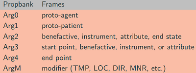
PropBank is a version of the Penn Treebank annotated with semantic roles. More coarse-grained than Frame Semantics:

End-to-end SRL system

基本的结构单元是Bi-LSTM，用法是： · a standard LSTM layer processes the input in forward direction; · the output of this LSTM layer is the input to another LSTM layer, but in reverse direction; 这些Bi-LSTM单元可以叠加起来构造更深层的神经网络.

The input (processed word by word) features are: • argument and predicate: the argument is the word being processed, the predicate is the word it depends on; • predicate context (ctx-p): the words around the predicate; also used to distinguish multiple instances of the same predicate; • region mark (m_r): indicates if the argument is in the predicate context region or not; • if a sequence has n_p predicates it is processed n_p times.

Output: semantic role label for the predicate/argument pair using IOB tags (inside, outside, beginning).

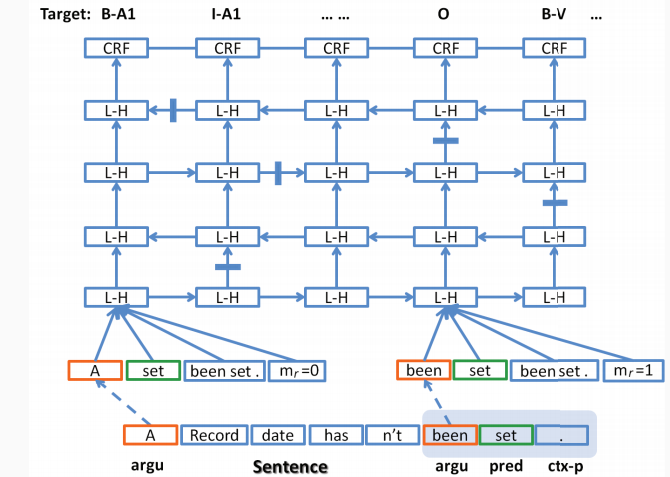
Training: • Word embeddings are used as input, not raw words; • the embeddings for arguments, predicate, and ctx-p, as well as m_r are concatenated and used as input for the Bi-LSTM; • the output is passed through a conditional random field (CRF); allows to model dependencies between output labels; • Viterbi decoding is used to compute the best output sequence

Model learns “syntax”(Maybe): it associates argument and predicate words using the forget gate:

Semantic Parsing

Semantic Parsing 指语义分析，把文本解析为任意的逻辑形式(一种 meaning representation)，比如 first-order logic(FOL). Sam likes Casey - likes(Sam, Casey); Anna's dog Mr. PeanutButter misses her - misses(MrPB, Anna) ∧ dog(MrPB); Kim likes everyone - ∀x.likes(x, Kim). Predicate-argument structure is a good match for FOL, as well as structures with argument-like elements (e.g. NPs). Determiners, quantifiers (e.g. “everyone”, “anyone”), and negation can be expressed in FOL.

However, much of natural language is unverifiable, ambiguous, non-canonical. That makes it hard to represent the wide-coverage meaning of arbitrary NL. Closed domains are easier, and can sometimes be harvested automatically, e.g. GEOQUERY dataset.

This leads to a proliferation of domain-specific MRs. · Pairs of NL sentences with structured MR can be collected, e.g. IFTTT dataset (Quirk et al. 2015). · WikiTableQuestions · Google’s knowledge graph

Viewing MR as a string, semantic parsing is just conditional language modeling. Trainable alternative to compositional approaches: encoder-decoder neural models. The encoder and decoder can be mixed and matched: RNN, top-down tree RNN.

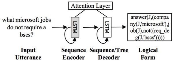
Works well on small, closed domains if we have training data, but there are many unsolved phenomena/ problems in semantics.

Abstract meaning representation (AMR)

• The edges (ARG0 and ARG1) are relations • Each node in the graph has a variable • They are labeled with concepts • d / dog means “d is an instance of dog” The dog is eating a bone (e / eat-01     :ARG0 (d / dog)     :ARG1 (b / bone))

The dog wants to eat the bone (want-01     :ARG0 (d / dog)     :ARG1 (e / eat-01         :ARG0 d         :ARG1 (b / bone)))

Coreference Charles just graduated, and now Bob wants Anna to give him a job. Q: who does him refer to?

Metonymy Westminster decided to distribute funds throughout England, Wales, Northern Island, and Scotland decided(Parliament, …)

Implicature That cake looks delicious - I would like a piece of that cake.

Even more phenomena… • Abbreviations (e.g. National Health Service=NHS) • Nicknames (JLaw=Jennifer Lawrence) • Metaphor (crime is a virus infecting the city) • Time expressions and change of state • Many others

TODO(指代消解 Coreference Resolution)

Unsupervised Part-of-Speech Tagging

Parts-of-speech(POS), word classes, or syntactic categories, 一般指八个词性：noun, verb, adjective, adverb, pronoun, preposition, conjunction, interjection, 有时候是 numeral, article or determiner. 1, noun 名詞 ( n. ) 2, pronoun 代名詞 ( pron. ) 3, verb 動詞 ( v. ) 4, adjective 形容詞 ( adj. ) 5, adverb 副詞 ( adv. ) 6, preposition 介系詞 ( prep. ) 7, conjunction 連接詞 ( conj. ) 8, interjection 感歎詞 ( int. )

Tagging is a task that take a sentence, assign each word a label indicating its syntactic category (part of speech).

One common standard label is Penn Treebank PoS tagset.

DT - Determiner 定语 IN - Preposition or subord. conjunction NN - Noun, singular or mass NNS - Noun, plural NNP - Proper noun, singular RB - Adverb TO - to VB - Verb, base form VBZ - Verb, 3rd person singular present

In supervised POS tagging, the input is the text and a set of allowed POS labels. The training data contains input and output examples. The output is a guess, for each word in the test data, which POS label it should have.

A common approach is to use an HMM. To train it, choose parameters θ that maximize $P(x,y \mid θ)$, the probability of the training data given the parameters. This is maximum likelihood estimation and it was covered in ANLP. You can use the model to predict y for each x in the test data by solving $P(y \mid x,θ)$ using the Viterbi algorithm.

A consequence of supervised training with MLE is that the model will only learn non-zero probability for tag-word pairs that actually appear in the data. Hence, if “the” is only ever tagged with DT in the training data, then the model will learn that the probability of producing “the” from any other tag is zero. This means that many word tokens will be (empirically) unambiguous, which is one of the things that makes supervised POS tagging easy.

RNNs 虽然也可以处理序列模型, 但是神经网络需要目标函数, 没有目标无法计算损失, 就无法调整参数, 也就是"监督学习".

Current PoS taggers are highly accurate (97% accuracy on Penn Treebank). But they require manually labelled training data, which for many major language is not available. Hence motivated for unsupervised PoS tagging.

In unsupervised POS tagging, the input is the text and the number of clusters. The training data contains only input examples. The output is a guess, for each word in the text, which cluster the word belongs to. For example:

Number of clusters: 50
Input x: The hungry cat meows
Output y: 23 45 7 18

What we hope is that the cluster labels will correlate with true POS labels; that is, that tokens labeled 23 will tend to be determiners, that clusters label 45 will tend to be adjectives, and so on.

这个时候可以使用隐马尔科夫模型, 这个"隐"就是针对没有目标可以参考这种情况.

Hidden Markov Models

The unsupervised tagging models here are based on Hidden Markov Models (HMMs). 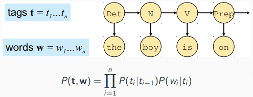To train it, choose parameters θ that maximize $P(x \mid θ)$, the probability of the training data given the parameters.

The parameters θ = (τ, ω) define: • τ : the probability distribution over tag-tag transitions; • ω: the probability distribution over word-tag outputs. The parameters are sets of multinomial distributions: • $ω = ω^{(1)} . . . ω^{(T)}$: the output distributions for each tag; • $τ = τ^{(1)} . . . τ^{(T)}$: the transition distributions for each tag; • $ω^{(t)} = ω_1^{(t)}. . . ω_W^{(t)}$: the output distribution from tag $t$; • $τ^{(t)} = τ_1^{(t)}. . . τ_T^{(t)}$: the transition distribution from tag $t$.

Another way to write the model, often used in statistics and machine learning:

$w_i | t_i = t ∼ Multinomial(ω^{(t)})$

So as tag, given that $t_{i−1} = t$, the value of $t_i$ is drawn from a multinomial distribution with parameters $τ^{(t)}$.

How to estimate ω and τ without supervision. This is still maximum likelihood estimation, but notice that it’s more difficult because the tags y are unobserved, so you must marginalize them out.

For estimation (i.e., training the model, determining its parameters), we need a procedure to set θ based on data. Rely on Bayes Rule: \begin{equation}\begin{split} P(θ|w)&=\frac{P(w|θ)P(θ)}{P(w)}\\ &∝P(w|θ)P(θ)\\ \end{split}\end{equation} Choose the θ that maximize the likelihood $P(w|θ)$. Basically, we ignore the prior. In most cases, this is equivalent to assuming a uniform prior.

To do this, you can use expectation maximization (EM), a variant of MLE that can cope with unobserved data, which was also covered in ANLP. For examples, forward-backward algorithm for HMMs, inside-outside algorithm for PCFGs, k-means clustering.

For inference (i.e., decoding, applying the model at test time), we need to know θ and then we can compute $P(t, w)$:

E-step: use current estimate of θ to compute expected counts of hidden events ($n(t,t^{\prime})$, $n(t,w)$). M-step: recompute θ using expected counts.

You can then use the trained model to predict y for each x in the test data by solving $P(y \mid x,θ)$ using the Viterbi algorithm.

But EM often fails, even very small amounts of training data have been show to work better than EM. One consequence of unsupervised training with EM is that every word can be assigned to any cluster label. This makes things really difficult, because it means every word is ambiguous. The basic assumptions of EM (that any tag-word or tag-tag distribution is equally likely) make this even more difficult.

Instead, use Bayesian HMM with Gibbs sampling.

Bayesian HMM

When training HMM model, we are not actually interested in the value of θ, we could simply integrate it out. This approach is called Bayesian integration. Integrating over θ gives us an average over all possible parameters values.

The Bayesian HMM is simply an alternative way to solve the unsupervised POS tagging problem. The input and output is the same. But instead of learning θ, we directly solve $P(y \mid x)$. Note that we don’t need to learn θ (though we could) - in this setting, we integrate it out, after first supplying some information about the tag-tag and word-tag distributions encoded in θ. Specifically, we tell the model that a sparse distribution is much more likely than a uniform distribution. We do this by defining a distribution $P(θ)$, and this gives us a new model, $P(y,x \mid θ)×P(θ)$. By integrating out θ we can solve the unsupervised tagging problem directly.

Example: we want to predict a spinner result will be “a” or not? • Parameter θ indicates spinner result: $P(θ = a) = .45$, $P(θ = b) = .35$, $P(θ = c) = .2$; • define t = 1: result is “a”, t = 0: result is not “a”; • make a prediction about one random variable (t) based on the value of another random variable (θ).

Maximum likelihood approach: choose most probable θ, $\hat{θ} = a$, and $P(t = 1|\hat{θ}) = 1$, so we predict $t = 1$.

Bayesian approach: average over θ, $P(t = 1) = \sum_θ P(t = 1|θ)P(θ) = 1(.45) + 0(.35) + 0(0.2) = .45$, predict t = 0.

Advantages of Bayesian integration: • accounts for uncertainty as to the exact value of θ; • models the shape of the distribution over θ; • increases robustness: there may be a range of good values of θ; • we can use priors favoring sparse solutions (more on this later).

Dirichlet distribution Choosing the right prior can make integration easier. A $K$-dimensional Dirichlet with parameters $α = α_1 . . . α_K$ is defined as:

$$ P(θ) = \frac{1}{Z} \prod_{j=1}^K θ_j^{α_j−1} $$

We usually only use symmetric Dirichlets, where $α_1 . . . α_K$ are all equal to β. We write Dirichlet(β) to mean $Dirichlet(β, . . . , β)$.

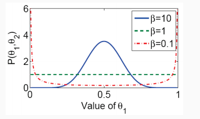注意到这是一个二维的概率密度图. $β>1$意味着更喜欢均值分布, 此时$θ$大概率落在$0.5$附近,因为$θ_1+θ_2=1$, 所以此时$θ_1, θ_2$概率均等. 如果$β=1$, $θ_1$的任何取值是等概率的, 等于说任何$θ_1,θ_2$的组合概率都是均等的.

To Bayesianize the HMM, we augment with it with symmetric Dirichlet priors:

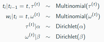
To simplify things, use a bigram version of the Bayesian HMM; If we integrate out the parameters θ = (τ, ω), we get:

Use these distributions to find $P(t|w)$ using an estimation method called Gibbs sampling.

Results: Integrating over parameters is useful in itself, even with uninformative priors $(α = β = 1)$;

总结： · Bayesian HMM improves performance by averaging out uncertainty; · allows us to use priors that favor sparse solutions as they occur in language data. · Using a tag dictionary is also really helpful. We still have no labeled training data, but if we only allow each word to be tagged with one of the labels that appears in the dictionary, then most word-tag pairs will have probability zero. So this is a very different way of supplying information to the unsupervised model that is very effective.

Bias in NLP

The social impact of NLP

Outcome of an NLP experiment can have a direct effect on people’s lives, e.g.

1. 频繁出现亚马逊 Alexa 突然发出诡异笑声，给多名用户造成困惑和恐慌, 因为人们谈话中偶然包含 trigger 词：“Alexa, laugh” 而发出 - 亚马逊的解决方案是把 trigger 改为更难触发的 “Alexa, can you laugh”
2. Chatbot 对于人们敏感问题的不恰当回答, 比如 “Should I kill myself?” - “Yes."，这些回答对患有心理障碍的人群或者青少年儿童带来非常大的危害。
3. Microsoft 的 AI chatbot 上线仅一天, 就通过 twitter 和人交谈并学会涉及种族, 性别歧视等的话语, 典型的 “garbage in, garbage out” 现象.
4. 其他涉及数据隐私等问题

语言的特性，导致NLP涉及的社会伦理问题非常多, 而且影响非常大： · 语言传递着信息、偏见，是政治性的、权力的工具, 同时比其他技术带有更明显的拟人化、人格化倾向，这可能给个人生活带来不便或危害，给整个社会带来舆论影响。 · Any dataset carries demographic bias: latent information about the demographics of the people that produced it. That excludes people from other demographics.

同时人类本身的认知容易加深偏见: The availability heuristic: the more knowledge people have about a specific topic, the more important they think it must be. Topic overexposure creates biases that can lead to discrimination and reinforcement of existing biases. E.g. NLP focused on English may be self-reinforcing.

NLP 实验本身容易加深偏见： • Advanced grammar analysis can improve search and educational NLP, but also reinforce prescriptive linguistic norms. • Stylometric analysis can help discover provenance of historical documents, but also unmask anonymous political dissenters.

NLP 技术可能被不恰当地使用： • Text classification and IR can help identify information of interest, but also aid censors. • NLP can be used to discriminate fake reviews and news, and also to generate them.

Word embeddings contain human-like biases

word2vec learns semantic/ syntactic relationships, also keep company with unsavoury stereotypes and biases? • Man:Woman - King:Queen • Man:Doctor - Woman:Nurse • Man:Computer Programmer - Woman:Homemaker

Measure bias using implicit association tests: 1, Compute similarity of group1 and stereotype1 word embeddings. Cosine similarity is use to measure association (in place of reaction time). 2, Compute similarity of group1 and stereotype 2 word embeddings. 3, Null hypothesis: if group1 is not more strongly associated to one of the stereotypes, there will be no difference in the means. 4, Effect size measured using Cohen’s d. 5, Repeat for group 2.

Experiments • Uses GloVe trained on Common Crawl—a large-scale crawl of the web. • Removed low frequency names. • Removed names that were least “name-like” (e.g. Will) algorithmically. • Each concept is represented using a small set of words, designed for previous experiments in the psychology literature.

Result: · flowers associate with pleasant, insects associate with unpleasant. $p < 10^{−7}$ · Men’s names associate with career, women’s names associate with family. $p < 10^{−3}$ · European American names associate with pleasant, African American names associate with unpleasant. $p < 10^{−8}$

这些结果的确真实地反映人类社会的现状。但大部分性别方面的偏见其实是反映了目前的社会分工，无所谓高低贵贱；人种的偏见倒是反映了历史问题对现在的影响，这种偏见是不符合道德的。人对于其他生物的偏见，虽然是没必要的，但人类的确倾向于喜爱行为"可爱”，外形"美好"的生物，比如大熊猫就是比鳄鱼受欢迎。

偏见的存在不一定合理。哪些偏见是不合理的，才是人们更应该去思考和讨论的地方。

Debiasing word embeddings

Bolukbasi. et. al., 2016. Man is to Computer Programmer as Woman is to Homemaker? Debiasing Word Embeddings提供了一个思路:

1. 确认偏见的方向
2. 中和抵消偏见: 对于非定性的词（如"医生"），通过投射来消除偏见
3. 等价：让father - mother和boy - girl等距，让定性词间的距离只有性别的距离；或者让doctor - woman和doctor - man等距，消除非定性词的性别偏见。

什么词需要抵消偏见: 训练一个线性分类器来确定词是非定性还是非定性的, 结果当然是大部分英语词都是非定性的.

If analogies reveal a gender dimension, use analogies on specific seed pairs to find it. 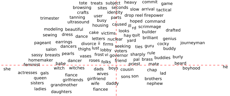y 轴下面的词属于定性词, 不需要中性化, 而y轴之上的词则需要进行中性化处理.

不同的偏见, 需要不同的 seed words; 一种偏见, 可以有多种 seed words 选择: 除了用"She-He"作为性别偏见的基准, 还有其他选择.

编码器—解码器 Sequence-to-sequence 和注意力机制

当输入输出都是不定长序列时, 比如机器翻译这种任务，需要使用 Sequence-to-sequence（seq2seq）或者 encoder-decoder 神经网络结构。这种结构可以通过一种方法叫注意力机制来显著提高性能。

编码器—解码器 Sequence-to-sequence（seq2seq）

编码器：所谓编码，就是把不定长的输入序列输入RNN，以得出某种定长的编码信息。 解码器：所谓解码，就是把编码器编码后的信息（一般取编码器的RNN最终时刻的隐含层变量）输入到解码器的RNN中，每个t时刻的输出既取决于之前时刻（t-1）的输出又取决于编码信息。等同于一个以解码信息作为条件概率生成目标语言句子的语言模型。

所以 seq2seq 本质是一个条件概率语言模型：语言模型是指解码器每次会预测下一个出现的单词，条件概率是指预测是基于编码后的源句子。

注意力

在传统的seq2seq模型中，解码器各个时刻都使用相同的编码信息，这就要求解码器把源输入序列的所有信息都解码并整合到最后时刻的隐含状态中，这个是很大的信息瓶颈。而人们知道，在实际任务中，比如机器翻译，目标句子的不同单词，一般只对应源句子的某一部分而已。如果能够让解码器在解码时，在不同时刻专注于源输入序列的不同部分，那么就可以突破这个瓶颈。

1. 对于解码器的每一时间步的隐含状态s_t，可以衡量其与编码器的所有时间步隐含状态h₀……e_t的相似性(或score评分) e = α(s, h)，简单的评分方式是元素间相乘, e = s*h（Bahanau的论文提供了更复杂的形式), 也可以参考论文Effective Approaches to Attention-based Neural Machine Translation探讨的集中评分方式, 这篇论文提供了一种 Bilinear 形式的相似性评分法, 就是在s和h之间以点乘的形式插入一个交互矩阵 interaction matrix.
2. 对得出的评分求加权平均a = softmax(e), 得出的权值分布也称注意力权重
3. 通过注意力权重把编码器隐含状态加权求和，得到注意力输出 A = Σah
4. 最后把注意力输出和对应时间步的解码器隐含状态s_t拼接在一起 [A;s_t]，作为解码器rnn的隐含层.