Links: https://arxiv.org/abs/2101.03961
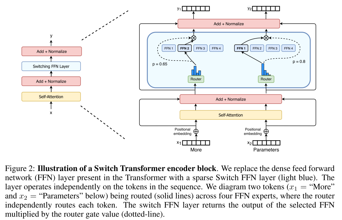
“SWITCH TRANSFORMERS: SCALING TO TRILLION PARAMETER MODELS WITH SIMPLE AND EFFICIENT SPARSITY”,提出了一种可以扩展到万亿参数的网络,有两个比较大的创新,基于Transformer MoE网络结构,简化了MoE的routing机制,降低了计算量;进一步通过数据并行+模型并行+expert并行的方式降低了训练通信量,提升训练性能。
模型

Simplifying Sparse Routing
- Mixture of Expert Routing which takes as an input a token representation x and then routes this to the best deter- mined top-k experts
- Switch Routing: route to only a single expert, this simplification preserves model quality, reduces routing computation and performs better.

Sparse routing通过参数Wr计算出一个在N个experts上的softmax分布,对每个token输入筛选概率最高的 top k 个 experts,对应的是MOE中的门控机制。这样对算力的需求并没有随着参数量的增加而大幅增长,使得这个模型更加容易训练。
EFFICIENT SPARSE ROUTING
并行Switch实现
- tensor shapes are statically determined at compilation time
- computation is dynamic due to the routing decisions at training and inference.
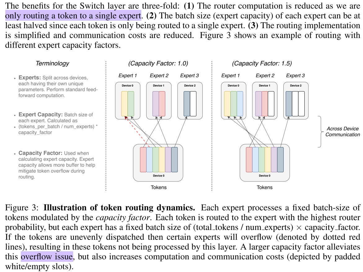
One important technical consideration is how to set the expert capacity - the number of tokens each expert computes: is set by evenly dividing the number of tokens in the batch across the number of experts, and then further expanding by a capacity factor,
$$\text { expert capacity }=\left(\frac{\text { tokens per batch }}{\text { number of experts }}\right) \times \text { capacity factor }$$- capacity factor > 1.0 create additional buffer to accommodate for when tokens are not perfectly balanced across experts.
- dropped tokens: If too many tokens are routed to an expert, computation is skipped and the token representation is passed directly to the next layer through the residual connection.
可微分负载均衡损失函数
为了均衡各个专家间的负载,需要一个辅助loss (Shazeer et al., 2017; 2018; Lepikhin et al., 2020)
For each Switch layer, this auxiliary loss is added to the total model loss during training
具体的,给定 N 个 experts (indexed by i = 1 to N),以及一个 batch $B$ with $T$ tokens, 设定一个辅助损失函数以 encourages uniform routing since it is minimized under a uniform distribution. the auxiliary loss is computed as the scaled dot-product between vectors f and P:
$$\operatorname{loss}=\alpha N \cdot \sum_{i=1}^{N} f_{i} \cdot P_{i}$$其中 $f_i$ is the fraction of tokens dispatched to expert i,
$$f_{i}=\frac{1}{T} \sum_{x \in \mathcal{B}} \mathbb{1}\{\operatorname{argmax} p(x), i\}$$大写的 $P_i$是可微分的, is the probability fraction to expert i across all tokens in the batch $B$
$$P_{i}=\frac{1}{T} \sum_{x \in \mathcal{B}} p_{i}(x)$$小写的$p_i(x)$ is the probability of routing token x to expert i.
$N$用于 keep the loss constant as the number of experts varies since under uniform routing
$\sum^N_1 (f_i ·P_i) = \sum^N_1( \frac{1}{N} · \frac{1}{N}) = \frac{1}{N}$.
$α = 10^{−2}$ to ensure load balancing while small enough to not to overwhelm the primary cross-entropy objective.
2.4 提升训练效果和fine-tuning的技巧
- 提升训练稳定性 - Selective precision with large sparse models
- 文章说明不需要全局使用float32,而是局部使用float32也可能保证稳定性
- cast the router input to float32 precision,the float32 precision is only used within the body of the router function,计算完再cast to bfloat16,然后才分发出去,避免了通信负担
- Smaller parameter initialization for stability, Reduced initialization scale improves stability. 在truncated normal distribution初始化基础上,reducing the default Transformer initialization scale s = 1.0 by a factor of 10.
- Regularizing large sparse models:increase the dropout inside the experts, which we name as expert dropout.
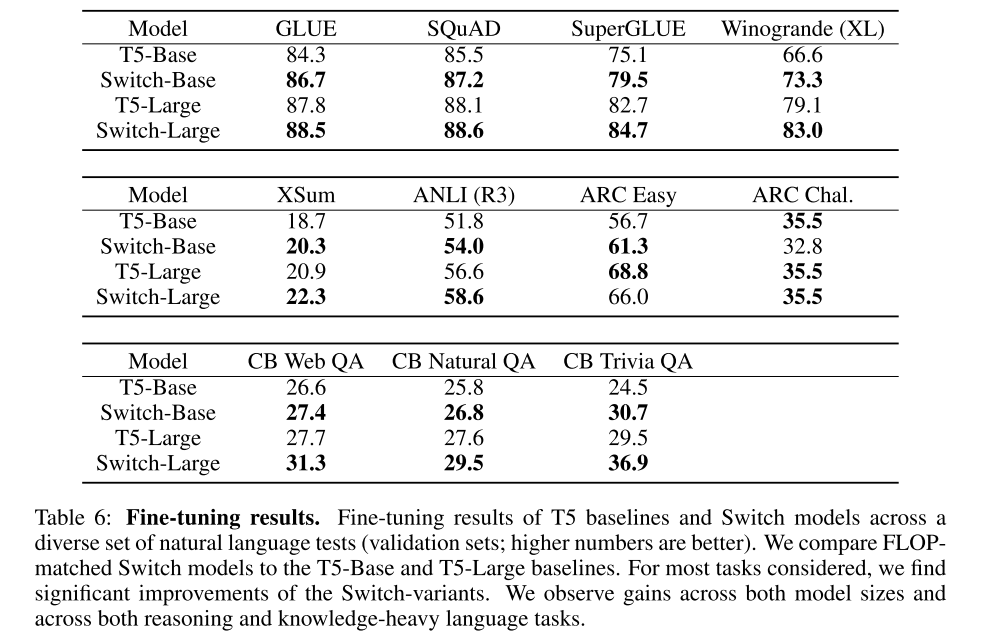
4 下游fine-tuning效果得到提升

5 DESIGNING MODELS WITH DATA, MODEL, AND EXPERT-PARALLELISM Arbitrarily
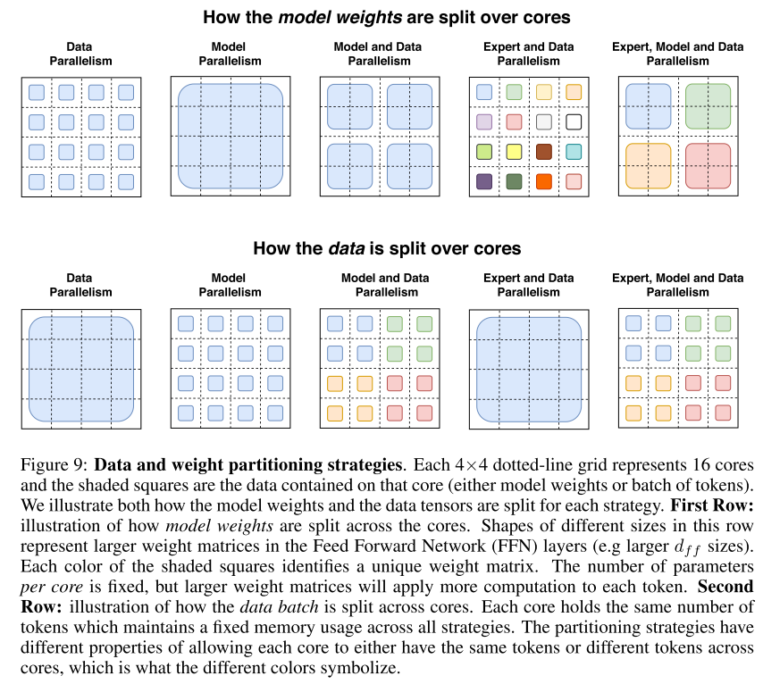
Switch Transformer用了多种并行策略,数据并行+模型并行+expert并行。
Expert并行实际上就是一种算子间的并行,experts在计算图上是个多并行子图分支,每个分支是一个FFNN结构。
在FFN内部,还可以进一步进行算子级的模型并行。每个FFN内部,the intermediate is $h = xW_{in}$ and then the output of the layer is $y = ReLU(h)W_{out}$. $W_{in}$ and $W_{out}$ are applied independently to each token and have sizes $[d_{model}, d_{ff}]$ and $[d_{ff}, d_{model}]$.
所以Switch Transformer的并行方式是数据并行+算子级模型并行+算子间模型并行,这种并行模型相较于数据并行+算子级模型并行的方式,在MoE网络结构上能够获得更低的通信开销,提高并行的效率。参照文章中的定义:
B - Number of tokens in the batch.
N - Number of total cores.
n - Number of ways for data-parallelism sharding. m - Number of ways for model-parallelism sharding.
E - Number of experts in Switch layers.
C - Expert capacity, the batch size of each expert.

数据并行:n = N,m = 1,数据分割到各个cores,模型完整地复制到各个cores,图9第一列, no communication is needed until the entire forward and backward pass is finished and the gradients need to be then aggregated across all cores
模型并行:n = 1,m = N,For each forward and backward pass, a communication cost is now incurred
数据和模型并行:N = n ×m cores,In the forward and backward pass each core communicates a tensor of size $[B/n, d_{model}]$ in an all-reduce operation.
Expert和数据并行:让E = n = N,对每个core分到的每个token,local router决定如何分配给不同的experts,输出是一个binary matrix $[n, B/n, E, C]$,Because each core has its own expert, we do an all-to-all communication of size $[E, C, d_{model}]$ to now shard the E dimension instead of the n-dimension.
Expert、模型和数据并行:在N cores资源固定的前提下,因为 $N = n \times m$, 只能在模型并行和数据并行,也就是batch-size和$d_{ff}$ size之间做trade-off. 文章在section5.6详细讨论这部分。