注意力机制的原理是计算query和每个key之间的相关性$\alpha_c(q,k_i)$以获得注意力分配权重。在大部分NLP任务中,key和value都是输入序列的编码。
注意力机制一般是用于提升seq2seq或者encoder-decoder架构的表现。但这篇2017 NIPS的文章Attention is all you need提出我们可以仅依赖注意力机制就可以完成很多任务. 文章的动机是LSTM这种时序模型速度实在是太慢了。
近些年来,RNN(及其变种 LSTM, GRU)已成为很多nlp任务如机器翻译的经典网络结构。RNN从左到右或从右到左的方式顺序处理语言。RNN的按顺序处理的性质也使得其更难以充分利用现代快速计算设备,例如GPU等优于并行而非顺序处理的计算单元。虽然卷积神经网络(CNN)的时序性远小于RNN,但CNN体系结构如ByteNet或ConvS2S中,糅合远距离部分的信息所需的步骤数仍随着距离的增加而增长。
因为一次处理一个单词,RNN需要处理多个时序的单词来做出依赖于长远离单词的决定。但各种研究和实验逐渐表明,决策需要的步骤越多,循环网络就越难以学习如何做出这些决定。而本身LSTM就是为了解决long term dependency问题,但是解决得并不好。很多时候还需要额外加一层注意力层来处理long term dependency。
所以这次他们直接在编码器和解码器之间直接用attention,这样句子单词的依赖长度最多只有1,减少了信息传输路径。他们称之为Transformer。Transformer只执行一小段constant的步骤(根据经验选择)。在encoder和decoder中,分别应用self-attention 自注意力机制(也称为intra Attention), 顾名思义,指的不是传统的seq2seq架构中target和source之间的Attention机制,而是source或者target自身元素之间的Attention机制。也就是说此时Query, Key和Value都一样, 都是输入或者输出的序列编码. 具体计算过程和其他attention一样的,只是计算对象发生了变化. Self-attention 直接模拟句子中所有单词之间的关系,不管它们之间的位置如何。比如子“I arrived at the bank after crossing the river”,要确定“bank”一词是指河岸而不是金融机构,Transformer可以学会立即关注“river”这个词并在一步之内做出这个决定。
Transformer总体架构
与过去流行的使用基于自回归网络的Seq2Seq模型框架不同:
- Transformer使用注意力来编码(不需要LSTM/CNN之类的)。
- 引入自注意力机制
- Multi-Headed Attention Mechanism: 在编码器和解码器中使用 Multi-Headed self-attention。
Transformer也是基于encoder-decoder的架构。具体地说,为了计算给定单词的下一个表示 - 例如“bank” - Transformer将其与句子中的所有其他单词进行比较。这些比较的结果就是其他单词的注意力权重。这些注意力权重决定了其他单词应该为“bank”的下一个表达做出多少贡献。在计算“bank”的新表示时,能够消除歧义的“river”可以获得更高的关注。将注意力权重用来加权平均所有单词的表达,然后将加权平均的表达喂给一个全连接网络以生成“bank”的新表达,以反映出该句子正在谈论的是“河岸”。
![]()
Transformer的编码阶段概括起来就是:
- 首先为每个单词生成初始表达或embeddings。这些由空心圆表示。
- 然后,对于每一个词, 使用自注意力聚合来自所有其他上下文单词的信息,生成参考了整个上下文的每个单词的新表达,由实心球表示。并基于前面生成的表达, 连续地构建新的表达(下一层的实心圆)对每个单词并行地重复多次这种处理。
Encoder的self-attention中, 所有Key, Value和Query都来自同一位置, 即上一层encoder的输出。
解码器类似,所有Key, Value和Query都来自同一位置, 即上一层decoder的输出, 不过只能看到上一层对应当前query位置之前的部分。生成Query时, 不仅关注前一步的输出,还参考编码器的最后一层输出。
![]()
N = 6, 这些“层”中的每一个由两个子层组成:position-wise FNN 和一个(编码器),或两个(解码器),基于注意力的子层。其中每个还包含4个线性投影和注意逻辑。
编码器:
- Stage 1 - 输入编码: 序列的顺序信息是非常重要的。由于没有循环,也没有卷积,因此使用“位置编码”表示序列中每个标记的绝对(或相对)位置的信息。
- positional encodings $\oplus$ embedded input
- Stage 2 – Multi-head self-attention 和 Stage 3 – position-wise FFN. 两个阶段都是用来残差连接, 接着正则化输出层
Stage1_out = Embedding512 + TokenPositionEncoding512
Stage2_out = layer_normalization(multihead_attention(Stage1_out) + Stage1_out)
Stage3_out = layer_normalization(FFN(Stage2_out) + Stage2_out)

out_enc = Stage3_out
解码器的架构类似,但它在第3阶段采用了附加层, 在输出层上的 mask multi-head attention:
- Stage 1 – 输入解码: 输入 output embedding,偏移一个位置以确保对位置
i的预测仅取决于< i的位置。
def shift_right_3d(x, pad_value=None):
  """Shift the second dimension of x right by one."""
  if pad_value is None:
    shifted_targets = tf.pad(x, [[0, 0], [1, 0], [0, 0]])[:, :-1, :]
  else:
    shifted_targets = tf.concat([pad_value, x], axis=1)[:, :-1, :]
  return shifted_targets
- Stage 2 - Masked Multi-head self-attention: 需要有一个mask来防止当前位置
i的生成任务看到后续> i位置的信息。
# 使用pytorch版本的教程中提供的范例
# http://nlp.seas.harvard.edu/2018/04/03/attention.html
def subsequent_mask(size):
    "Mask out subsequent positions."
    attn_shape = (1, size, size)
    subsequent_mask = np.triu(np.ones(attn_shape), k=1).astype('uint8')
    return torch.from_numpy(subsequent_mask) == 0

# # The attention mask shows the position each tgt word (row) is allowed to look at (column).
# Words are blocked for attending to future words during training.
plt.figure(figsize=(5,5))
plt.imshow(subsequent_mask(20)[0])
![]()
阶段2,3和4同样使用了残差连接,然后在输出使用归一化层。
Stage1_out = OutputEmbedding512 + TokenPositionEncoding512

Stage2_Mask = masked_multihead_attention(Stage1_out)
Stage2_Norm1 = layer_normalization(Stage2_Mask) + Stage1_out
Stage2_Multi = multihead_attention(Stage2_Norm1 + out_enc) +  Stage2_Norm1
Stage2_Norm2 = layer_normalization(Stage2_Multi) + Stage2_Multi

Stage3_FNN = FNN(Stage2_Norm2)
Stage3_Norm = layer_normalization(Stage3_FNN) + Stage2_Norm2

out_dec = Stage3_Norm
可以利用开源的Tensor2Tensor,通过调用几个命令来训练Transformer网络进行翻译和解析。
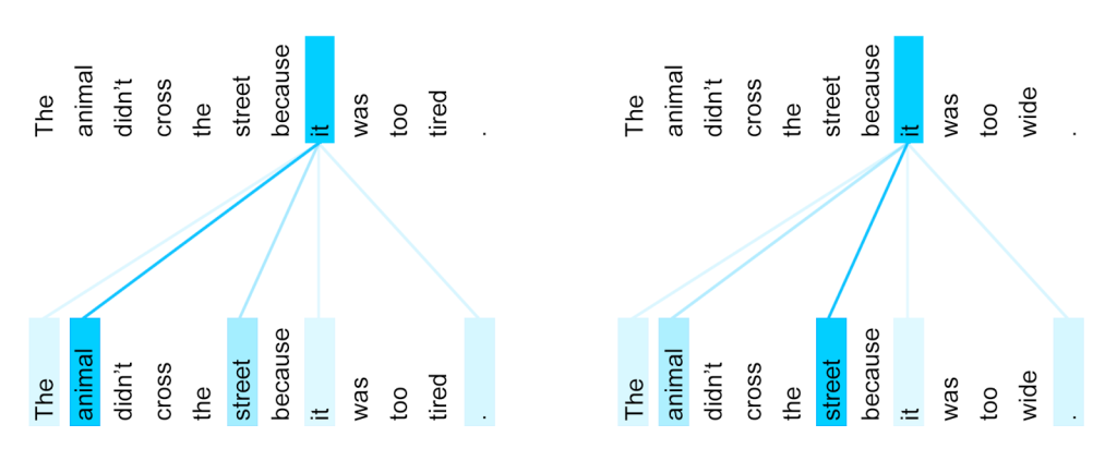
通过Self Attention对比Attention有什么增益呢?可以看到,自注意力算法可以捕获同一个句子中单词之间的语义特征, 比如共指消解(coreference resolution),例如句子中的单词“it”可以根据上下文引用句子的不同名词。除此之外, 理论上也可以捕捉一些语法特征. 
其实在LSTM_encoder-LSTM_decoder架构上的Attention也可以做到相同的操作, 但效果却不太好. 问题可能在于此时的Attention处理的不是纯粹的一个个序列编码, 而是经过LSTM(复杂的门控记忆与遗忘)编码后的包含前面时间步输入信息的一个个序列编码, 这个导致Attention的软寻址难度增大. 而现在是2019年, 几乎主流的文本编码方案都转投Transformer了, 可见单纯利用self-attention编码其实效率更高.
Attention
Vaswani, 2017明确定义了使用的注意力算法
$$\begin{eqnarray} Attention (Q,K,V) = softmax \Big( \frac{QK^T}{\sqrt{d_k}} \Big) V \end{eqnarray},$$其中$\mathbb{Q}\in\mathbb{R}^{n\times d_k}, \mathbb{K}\in\mathbb{R}^{m\times d_k}, \mathbb{V}\in\mathbb{R}^{m\times d_v}$. 这就是传统的Scaled Dot-Product Attention, 把这个Attention理解为一个神经网络层,将$n\times d_k$的序列$Q$编码成了一个新的$n\times d_v$的序列。因为对于较大的$d_k$,内积会数量级地放大, 太大的话softmax可能会被推到梯度消失区域, softmax后就非0即1(那就是hardmax), 所以$q \cdot k = \sum_{i=1}^{d_k}q_i k_i$按照比例因子$\sqrt{d_k}$缩放.
BERT/ALBERT中的点积attention实现:
# dot_product_attention from bert implementation
def dot_product_attention(q, k, v, bias, dropout_rate=0.0):
  """Dot-product attention.
  Args:
    q: Tensor with shape [..., length_q, depth_k].
    k: Tensor with shape [..., length_kv, depth_k]. Leading dimensions must
      match with q.
    v: Tensor with shape [..., length_kv, depth_v] Leading dimensions must
      match with q.
    bias: bias Tensor (see attention_bias())
    dropout_rate: a float.
  Returns:
    Tensor with shape [..., length_q, depth_v].
  """
  logits = tf.matmul(q, k, transpose_b=True)  # [..., length_q, length_kv]
  logits = tf.multiply(logits, 1.0 / math.sqrt(float(get_shape_list(q)[-1])))
  if bias is not None:
    # `attention_mask` = [B, T]
    from_shape = get_shape_list(q)
    if len(from_shape) == 4:
      broadcast_ones = tf.ones([from_shape[0], 1, from_shape[2], 1], tf.float32)
    elif len(from_shape) == 5:
      # from_shape = [B, N, Block_num, block_size, depth]#
      broadcast_ones = tf.ones([from_shape[0], 1, from_shape[2], from_shape[3],
                                1], tf.float32)

    bias = tf.matmul(broadcast_ones,
                     tf.cast(bias, tf.float32), transpose_b=True)

    # Since attention_mask is 1.0 for positions we want to attend and 0.0 for
    # masked positions, this operation will create a tensor which is 0.0 for
    # positions we want to attend and -10000.0 for masked positions.
    adder = (1.0 - bias) * -10000.0

    # Since we are adding it to the raw scores before the softmax, this is
    # effectively the same as removing these entirely.
    logits += adder
  else:
    adder = 0.0

  attention_probs = tf.nn.softmax(logits, name="attention_probs")
  attention_probs = dropout(attention_probs, dropout_rate)
  return tf.matmul(attention_probs, v)
# 使用pytorch版本的教程中提供的范例
# http://nlp.seas.harvard.edu/2018/04/03/attention.html
def attention(query, key, value, mask=None, dropout=0.0):
  "Compute 'Scaled Dot Product Attention'"
  d_k = query.size(-1)
  scores = torch.matmul(query, key.transpose(-2, -1)) \
           / math.sqrt(d_k)
  if mask is not None:
      scores = scores.masked_fill(mask == 0, -1e9)
  p_attn = F.softmax(scores, dim = -1)
  # (Dropout described below)
  p_attn = F.dropout(p_attn, p=dropout)
  return torch.matmul(p_attn, value), p_attn
这只是注意力的一种形式,还有其他比如query跟key的运算方式是拼接后再内积一个参数向量,权重也不一定要归一化,等等。
Self-Attention (SA)
在实际的应用中, 不同的场景的$Q,K,V$是不一样的, 如果是SQuAD的话,$Q$是文章的向量序列,$K=V$为问题的向量序列,输出就是Aligned Question Embedding。
Google所说的自注意力(SA), 就是$Attention(\mathbb{X},\mathbb{X},\mathbb{X})$, 通过在序列自身做Attention,寻找序列自身内部的联系。Google论文的主要贡献之一是它表明了SA在序列编码部分是相当重要的,甚至可以替代传统的RNN(LSTM), CNN, 而之前关于Seq2Seq的研究基本都是关注如何把注意力机制用在解码部分。
编码时,自注意力层处理来自相同位置的输入$queries, keys, value$,即编码器前一层的输出。编码器中的每个位置都可以关注前一层的所有位置.
在解码器中,SA层使每个位置能够关注解码器中当前及之前的所有位置。为了保持 auto-regressive 属性,需要阻止解码器中的向左信息流, 所以要在scaled dot-product attention层中屏蔽(设置为-∞)softmax输入中与非法连接相对应的所有值.
作者使用SA层而不是CNN或RNN层的动机是:
- 最小化每层的总计算复杂度: SA层通过$O(1)$数量的序列操作连接所有位置. ($O(n)$ in RNN)
- 最大化可并行化计算:对于序列长度$n$ < representation dimensionality $d$(对于SOTA序列表达模型,如word-piece, byte-pair)。对于非常长的序列$n > d$, SA可以仅考虑以相应输出位置为中心的输入序列中的某个大小$r$的邻域,从而将最大路径长度增加到$O(n/r)$
- 最小化由不同类型层组成的网络中任意两个输入和输出位置之间的最大路径长度。任何输入和输出序列中的位置组合之间的路径越短,越容易学习长距离依赖。
Multi-head Attention
Transformer的SA将关联输入和输出序列中的(特别是远程)位置的计算量减少到$O(1)$。然而,这是以降低有效分辨率为代价的,因为注意力加权位置被平均了。为了弥补这种损失, 文章提出了 Multi-head Attention:
- $h=8$ attention layers (“heads”): 将key $K$ 和 query $Q$ 线性投影到 $d_k$ 维度, 将value $V$ 投影到$d_v$维度, (线性投影的目的是减少维度) $$head_i = Attention(Q W^Q_i, K W^K_i, V W^V_i) , i=1,\dots,h$$ 投影是参数矩阵$W^Q_i, W^K_i\in\mathbb{R}^{d_{model}\times d_k}, W^V_i\in\mathbb{R}^{d_{model}\times d_v}$ $d_k=d_v=d_{model}/h = 64$
- 每层并行地应用 scaled-dot attention(用不同的线性变换), 得到$d_v$维度的输出
- 把每一层的输出拼接在一起 $Concat(head_1,\dots,head_h)$
- 再线性变换上一步的拼接向量$MultiHeadAttention(Q,K,V) = Concat(head_1,\dots,head_h) W^O$, where $W^0\in\mathbb{R}^{d_{hd_v}\times d_{model}}$
因为Transformer只是把原来$d_{model}$维度的注意力函数计算并行分割为$h$个独立的$d_{model}/h$维度的head, 所以计算量相差不大.
BERT/ALBERT中的multi-head attention层实现:
def attention_layer(from_tensor,
                    to_tensor,
                    attention_mask=None,
                    num_attention_heads=1,
                    query_act=None,
                    key_act=None,
                    value_act=None,
                    attention_probs_dropout_prob=0.0,
                    initializer_range=0.02,
                    batch_size=None,
                    from_seq_length=None,
                    to_seq_length=None):
  """Performs multi-headed attention from `from_tensor` to `to_tensor`.
  Args:
    from_tensor: float Tensor of shape [batch_size, from_seq_length,
      from_width].
    to_tensor: float Tensor of shape [batch_size, to_seq_length, to_width].
    attention_mask: (optional) int32 Tensor of shape [batch_size,
      from_seq_length, to_seq_length]. The values should be 1 or 0. The
      attention scores will effectively be set to -infinity for any positions in
      the mask that are 0, and will be unchanged for positions that are 1.
    num_attention_heads: int. Number of attention heads.
    query_act: (optional) Activation function for the query transform.
    key_act: (optional) Activation function for the key transform.
    value_act: (optional) Activation function for the value transform.
    attention_probs_dropout_prob: (optional) float. Dropout probability of the
      attention probabilities.
    initializer_range: float. Range of the weight initializer.
    batch_size: (Optional) int. If the input is 2D, this might be the batch size
      of the 3D version of the `from_tensor` and `to_tensor`.
    from_seq_length: (Optional) If the input is 2D, this might be the seq length
      of the 3D version of the `from_tensor`.
    to_seq_length: (Optional) If the input is 2D, this might be the seq length
      of the 3D version of the `to_tensor`.
  Returns:
    float Tensor of shape [batch_size, from_seq_length, num_attention_heads,
      size_per_head].
  Raises:
    ValueError: Any of the arguments or tensor shapes are invalid.
  """
  from_shape = get_shape_list(from_tensor, expected_rank=[2, 3])
  to_shape = get_shape_list(to_tensor, expected_rank=[2, 3])
  size_per_head = int(from_shape[2]/num_attention_heads)

  if len(from_shape) != len(to_shape):
    raise ValueError(
        "The rank of `from_tensor` must match the rank of `to_tensor`.")

  if len(from_shape) == 3:
    batch_size = from_shape[0]
    from_seq_length = from_shape[1]
    to_seq_length = to_shape[1]
  elif len(from_shape) == 2:
    if (batch_size is None or from_seq_length is None or to_seq_length is None):
      raise ValueError(
          "When passing in rank 2 tensors to attention_layer, the values "
          "for `batch_size`, `from_seq_length`, and `to_seq_length` "
          "must all be specified.")

  # Scalar dimensions referenced here:
  #   B = batch size (number of sequences)
  #   F = `from_tensor` sequence length
  #   T = `to_tensor` sequence length
  #   N = `num_attention_heads`
  #   H = `size_per_head`

  # `query_layer` = [B, F, N, H]
  q = dense_layer_3d(from_tensor, num_attention_heads, size_per_head,
                     create_initializer(initializer_range), query_act, "query")

  # `key_layer` = [B, T, N, H]
  k = dense_layer_3d(to_tensor, num_attention_heads, size_per_head,
                     create_initializer(initializer_range), key_act, "key")
  # `value_layer` = [B, T, N, H]
  v = dense_layer_3d(to_tensor, num_attention_heads, size_per_head,
                     create_initializer(initializer_range), value_act, "value")
  q = tf.transpose(q, [0, 2, 1, 3])
  k = tf.transpose(k, [0, 2, 1, 3])
  v = tf.transpose(v, [0, 2, 1, 3])
  if attention_mask is not None:
    attention_mask = tf.reshape(
        attention_mask, [batch_size, 1, to_seq_length, 1])
    # 'new_embeddings = [B, N, F, H]'
  new_embeddings = dot_product_attention(q, k, v, attention_mask,
                                         attention_probs_dropout_prob)

  return tf.transpose(new_embeddings, [0, 2, 1, 3])
可以看到k和v都是to_tensor.
# 使用pytorch版本的教程中提供的范例
# http://nlp.seas.harvard.edu/2018/04/03/attention.html
class MultiHeadedAttention(nn.Module):
  def __init__(self, h, d_model, dropout=0.1):
    "Take in model size and number of heads."
    super(MultiHeadedAttention, self).__init__()
    assert d_model % h == 0
    # We assume d_v always equals d_k
    self.d_k = d_model // h
    self.h = h
    self.p = dropout
    self.linears = clones(nn.Linear(d_model, d_model), 4)
    self.attn = None

  def forward(self, query, key, value, mask=None):
    if mask is not None:
      # Same mask applied to all h heads.
      mask = mask.unsqueeze(1)
    nbatches = query.size(0)

    # 1) Do all the linear projections in batch from d_model => h x d_k
    query, key, value = [l(x).view(nbatches, -1, self.h, self.d_k).transpose(1, 2)
                         for l, x in zip(self.linears, (query, key, value))]

    # 2) Apply attention on all the projected vectors in batch.
    x, self.attn = attention(query, key, value, mask=mask, dropout=self.p)

    # 3) "Concat" using a view and apply a final linear.
    x = x.transpose(1, 2).contiguous().view(nbatches, -1, self.h * self.d_k)
    return self.linears[-1](x)
NMT中Transformer以三种不同的方式使用Multi-head Attention:
- 在
encoder-decoder attention层中,queries来自前一层decoder层,并且 memory keys and values 来自encoder的输出。这让decoder的每个位置都可以注意到输入序列的所有位置。这其实还原了典型的seq2seq模型里常用的编码器 - 解码器注意力机制(例如Bahdanau et al., 2014或Conv2S2)。 - 编码器本身也包含了self-attention layers。在self-attention layers中,所有 keys, values and queries 来自相同的位置,在这里是编码器中前一层的输出。这样,编码器的每个位置都可以注意到前一层的所有位置。
with tf.variable_scope("attention_1"):
    with tf.variable_scope("self"):
      attention_output = attention_layer(
          from_tensor=layer_input,
          to_tensor=layer_input,
          attention_mask=attention_mask,
          num_attention_heads=num_attention_heads,
          attention_probs_dropout_prob=attention_probs_dropout_prob,
          initializer_range=initializer_range)
- 类似地,解码器中的 self-attention layers 允许解码器的每个位置注意到解码器中包括该位置在内的所有前面的位置(有mask屏蔽了后面的位置)。需要阻止解码器中的向左信息流以保持
自回归属性(auto-regressive 可以简单理解为时序序列的特性, 只能从左到右, 从过去到未来)。我们通过在scaled dot-product attention层中屏蔽(设置为-∞)softmax输入中与非法连接相对应的所有值来维持该特性。
Position-wise Feed-Forward Networks
在编码器和解码器中,每个层都包含一个全连接的前馈网络(FFN),FFN 分别应用于每个位置,使用相同的两个线性变换和一个ReLU
$$FFN(x) = max(0, xW_1+b_1) W_2 + b_2$$虽然线性变换在不同位置上是相同的,但它们在层与层之间使用不同的参数。它的工作方式类似于两个内核大小为1的卷积层. 输入/输出维度是$d_{model}=512$, 内层的维度$d_{ff} = 2048$.
# 使用pytorch版本的教程中提供的范例
# http://nlp.seas.harvard.edu/2018/04/03/attention.html
class PositionwiseFeedForward(nn.Module):
  "Implements FFN equation."
  def __init__(self, d_model, d_ff, dropout=0.1):
    super(PositionwiseFeedForward, self).__init__()
    # Torch linears have a `b` by default.
    self.w_1 = nn.Linear(d_model, d_ff)
    self.w_2 = nn.Linear(d_ff, d_model)
    self.dropout = nn.Dropout(dropout)

  def forward(self, x):
    return self.w_2(self.dropout(F.relu(self.w_1(x))))
Positional Encoding
在解码时序信息时,LSTM模型通过时间步的概念以输入/输出流一次一个的形式编码的. 而Transformer选择把时序编码为正弦波。这些信号作为额外的信息加入到输入和输出中以表达时序信息.
这种编码使模型能够感知到当前正在处理的是输入(或输出)序列的哪个部分。位置编码可以学习或者使用固定参数。作者进行了测试(PPL,BLEU),显示两种方式表现相似。文中作者选择使用固定的位置编码参数:
$$ \begin{eqnarray} PE_{(pos,2i)} = sin(pos/10000^{2i/d_{model}}) \end{eqnarray} $$$$ \begin{eqnarray} PE_{(pos,2i+1)} = cos(pos/10000^{2i/d_{model}})\end{eqnarray} $$其中$pos$是位置,$i$是维度。
也就是说,位置编码的每个维度对应于正弦余弦曲线的拼接。波长形成从2π到10000⋅2π的几何级数。选择这个函数,是因为假设它能让模型容易地学习相对位置,因为对于任意固定偏移$k$,$PE_{pos + k}$可以表示为$PE_{pos}$的线性函数。
# 使用pytorch版本的教程中提供的范例
# http://nlp.seas.harvard.edu/2018/04/03/attention.html
class PositionalEncoding(nn.Module):
  "Implement the PE function."
  def __init__(self, d_model, dropout, max_len=5000):
    super(PositionalEncoding, self).__init__()
    self.dropout = nn.Dropout(p=dropout)

    # Compute the positional encodings once in log space.
    pe = torch.zeros(max_len, d_model)
    position = torch.arange(0, max_len).unsqueeze(1)
    div_term = torch.exp(torch.arange(0, d_model, 2) *
                         -(math.log(10000.0) / d_model))
    pe[:, 0::2] = torch.sin(position * div_term)
    pe[:, 1::2] = torch.cos(position * div_term)
    pe = pe.unsqueeze(0)
    self.register_buffer('pe', pe)

  def forward(self, x):
    x = x + Variable(self.pe[:, :x.size(1)], requires_grad=False)
    return self.dropout(x)
位置编码将根据位置添加正弦余弦波。每个维度的波的频率和偏移是不同的。
plt.figure(figsize=(15, 5))
pe = PositionalEncoding(20, 0)
y = pe.forward(Variable(torch.zeros(1, 100, 20)))
plt.plot(np.arange(100), y[0, :, 4:8].data.numpy())
plt.legend(["dim %d"%p for p in [4,5,6,7]])
![]() 直观的理解是,将这些值添加到embedding中,一旦它们被投影到$Q / K / V$向量和dot product attention中,就给embedding向量之间提供了有意义的相对距离。
直观的理解是,将这些值添加到embedding中,一旦它们被投影到$Q / K / V$向量和dot product attention中,就给embedding向量之间提供了有意义的相对距离。
![]()
![]()
Shared-Weight Embeddings and Softmax
与其他序列转导模型类似,使用可学习的Embeddings将 input tokens and output tokens 转换为维度$d_{model}$的向量。通过线性变换和softmax函数将解码器的输出向量转换为预测的token概率。在Transformer模型中,两个嵌入层和pre-softmax线性变换之间共享相同的权重矩阵,在Embeddings层中,将权重乘以$\sqrt{d_{\text{model}}}$. 这些都是当前主流的操作。
# 使用pytorch版本的教程中提供的范例
# http://nlp.seas.harvard.edu/2018/04/03/attention.html
class Embeddings(nn.Module):
  def __init__(self, d_model, vocab):
    super(Embeddings, self).__init__()
    self.lut = nn.Embedding(vocab, d_model)
    self.d_model = d_model

  def forward(self, x):
    return self.lut(x) * math.sqrt(self.d_model)
启发
作者已经进行了一系列测试(论文表3),其中他们讨论N = 6层的建议,模型大小为512,基于h = 8个heads,键值维度为64,使用100K步。
还指出,由于模型质量随着$d_k$(行B)的减小而降低,因此可以进一步优化点积兼容性功能。
其声称提出的固定正弦位置编码,与学习到的位置编码相比,产生几乎相等的分数。
算法适合哪些类型的问题?
- 序列转导(语言翻译)
- 语法选区解析的经典语言分析任务 syntactic constituency parsing
- 共指消解 coreference resolution
参考资料
https://research.googleblog.com/2017/08/transformer-novel-neural-network.html https://research.googleblog.com/2017/06/accelerating-deep-learning-research.html https://mchromiak.github.io/articles/2017/Sep/12/Transformer-Attention-is-all-you-need/ http://nlp.seas.harvard.edu/2018/04/03/attention.html