时序决策
以经典的Atari游戏为例,agent在t时刻观测一段包含M个帧的视频$s_t = (x_{t-M+1}, ..., x_t) \in S$, 然后agent做决策, 决策是选择做出一个动作 $a_t \in A = \{ 1, ..., |A| \}$(A为可选的离散动作空间 ), 这个动作会让agent获得一个奖励$r_t$.
这就是时序决策过程, 是一个通用的决策框架,可以建模各种时序决策问题,例如游戏,机器人等. Agent 观察环境,基于policy $\pi\left(a_{t} \mid s_{t}\right)$ 做出响应动作,其中 $s_{t}$是当前环境的观察值(Observation 是环境State对Agent可见的部分)。Action会获得新的 Reward $r_{t+1}$, 以及新的环境反馈 $s_{t+1}$.
Note: It is important to distinguish between the state of the environment and the observation, which is the part of the environment state that the agent can see, e.g. in a poker game, the environment state consists of the cards belonging to all the players and the community cards, but the agent can observe only its own cards and a few community cards. In most literature, these terms are used interchangeably and observation is also denoted as .
Agent的目标是通过优化 policy来最大化期望奖励(未来的奖励相对于当前时间需要打折, 也就是贴现, 跟未来现金流贴现一个道理), 称之为 discounted return $R_t = \sum_{\tau=t}^{\infty} \gamma^{\tau-t} r_{\tau}$, $\gamma \in [0, 1]$就是贴现率.
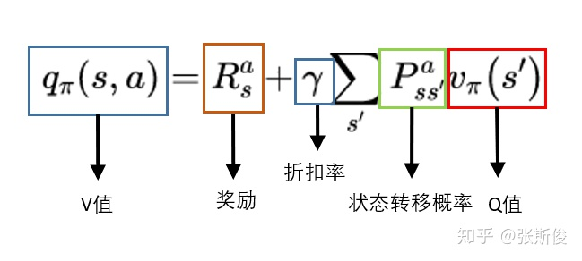
- 定义一个值 $Q^\pi(s, a)$, 用于表示一个 state-action pair $(s, a)$ 的价值, $Q^{\pi}(s,a)=E{\[R_t|s_t=s, a_t=a, \pi\]}$
- 定义$V^\pi(s)$用于表示状态$s$的价值 $V^{\pi}(s)=E_{a \sim \pi(s)}\[Q^{\pi}(s, a)\]$
为了计算Q值, 需要利用动态规划递归求解
$$Q^{\pi}(s, a)=E_{s^{\prime}}\[r+\gamma E_{a^{\prime} \sim \pi\left(s^{\prime}\right)}\[Q^{\pi}\left(s^{\prime}, a^{\prime}\right)\] \mid s, a, \pi\]$$最优的Q值就是 $Q^∗(s, a) = \max_{\pi} Q^\pi(s, a)$, 假设每次都选择能让当前Q最大的动作(这种方式是deterministic policy, 其他的还有Stochastic policies), $a = argmax_{a' \in A} Q^∗(s, a')$, 那么$V^∗(s) = \max_a Q^∗(s, a)$, 由此引出最优 $Q^{*}(s, a)$ 满足Bellman optimality equation
$$Q^*(s, a)=E_{s'}\[r+\gamma \max _{a^{\prime}} Q^{*}\left(s^{\prime}, a^{\prime}\right)\]$$The Cartpole Environment
The Cartpole Environment 是 RL中的Hello World. The environment simulates balancing a pole on a cart. The agent can nudge the cart left or right; these are the actions. It represents the state with a position on the x-axis, the velocity of the cart, the velocity of the tip of the pole and the angle of the pole (0° is straight up). The agent receives a reward of 1 for every step taken. The episode ends when the pole angle is more than ±12°, the cart position is more than ±2.4 (the edge of the display) or the episode length is greater than 200 steps. To solve the environment you need an average reward greater than or equal to 195 over 100 consecutive trials.
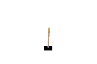
Observation $s_{t}$: 4D vector [position, velocity, angle, angular velocity]
Actions $a_{t}$: push the cart right (+1) or left (-1).
Reward $r_{t+1}$:
- 1 for every timestep that the pole remains upright.
- The episode ends when one of the following is true:
- the pole tips over some angle limit
- the cart moves outside of the world edges
- 200 time steps pass.
Goal: Learn policy $\pi\left(a_{t} \mid s_{t}\right)$ to maximize the sum of rewards in an episode $\sum_{t=0}^{T} \gamma^{t} r_{t}$.
$\gamma$ is a discount factor in [0, 1] that discounts future rewards relative to immediate rewards. This parameter helps us focus the policy, making it care more about obtaining rewards quickly.
Markov Decision Processes
MDP框架用于表达agent的学习过程,包含actions-rewards
A Markov Decision Process is defined by 5 components:
- A set of possible states
- An initial state
- A set of actions
- A transition model
- probability of transition $P(s'|s, a)$
- A reward function: $R(s'|s, a)$
- Discount $\gamma$: In this regard, the discount factor for a Markov Decision Process plays a similar role to a discount factor in Finance as it reflects the time value of rewards. This means that it is preferable to get a larger reward now and a smaller reward later, than it is to get a small reward now and a larger reward later due to the value of time.
Markov process from Wikipedia:
A stochastic process has the Markov property if the conditional probability distribution of future states of the process (conditional on both past and present states) depends only upon the present state, not on the sequence of events that preceded it. A process with this property is called a Markov process.
A Markov decision process provides a mathematical framework for modeling decision making in situations where outcomes are partly random and partly under the control of a decision maker.
there are two possible types of environments:
- The first is an environment that is completely observable, in which case its dynamics can be modeled as a Markov Process. Markov processes are characterized by a short-term memory, meaning the future depends not on the environments whole history, but instead only on the current state.
- The second type is a partially observed environment where some variables are not observable. These situations can be modeled using dynamic latent variable models, for example, using Hidden Markov models.
Decision Policies
Since the problem needs to be solved now, but the actions will be performed in the future, we need to define a decision policy.
The decision policy is a function that takes the current state S and translates it into an action A.
Deterministic policies:
- Always gives the same answer for a given state
- In general, it can depend on previous states and actions
- For a MDP, deterministic policies depend only on the current state, because state transitions also depend only on the current state
Stochastic (randomized) policies:
- Generalize deterministic policies
- For a MDP with known transition probabilities, we only need to consider deterministic policies
- If the transition probability is not known, randomization of actions allow exploration for a better estimation of the model
- Stochastic policies may work better than deterministic policies for a Partially Observed MDP (POMDP)
Exploration-Exploitation Dilemma
This concept is specific to reinforcement learning and does not arise in supervised or unsupervised Learning.
- Exploration means the agent is exploring potential hypotheses for how to choose actions, which inevitably will lead to some negative reward from the environment.
- Exploitation means how the agent exploits the limited knowledge about what it has already learned
This is referred to as a dilemma because at each time-step, the agent must decide whether it should explore or exploit in this state - but it can’t do both at once.
Reinforcement learning should ideally combine both exploration and exploitation, for example by switching between each one at different time steps.
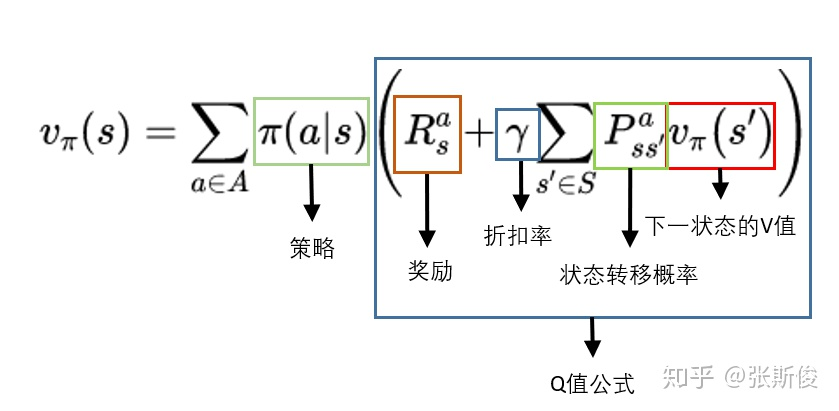
Q和V转换
$V$跟策略有很大关系,计算过程是:
- 从$S_i$出发,多次采样;
- 每个采样按照当前的 策略 选择行为$A_{i+1}$;
- 每个采样一直走到最终状态,并计算一路上获得的所有奖励总和;
- 计算每个采样获得的平均值, 这个平均值就是要求的$V$值。
$Q$的计算过程和$V$差不多,但是跟策略没有直接关系,而是与环境的状态转移概率相关,而环境的状态转移概率是不变的。
可以把采样过程形象化为有Markov过程生成的树,每个状态和动作都是一个树节点,而树的叶子节点就是结束状态。状态节点和动作节点是分层相隔的,所以Q和V可以相互换算,即每一层的Q可以由下一层的V计算出来,反之亦然。
What is the Q function and what is the V function in reinforcement learning?
$$\begin{align} v_{\pi}(s)&=E{\[G_t|S_t=s\]} \\\\ &=\sum_{g_t} p(g_t|S_t=s)g_t \\\\ &= \sum_{g_t}\sum_{a}p(g_t, a|S_t=s)g_t \\\\ &= \sum_{a}p(a|S_t=s)\sum_{g_t}p(g_t|S_t=s, A_t=a)g_t \\\\ &= \sum_{a}p(a|S_t=s)E{\[G_t|S_t=s, A_t=a\]} \\\\ &= \sum_{a}p(a|S_t=s)q_{\pi}(s,a) \end{align}$$一个状态的V值,就是这个状态下的所有动作的Q值$q_{\pi}(s,a)$ 在策略$p(a|S_t=s)$下的期望。
if we have a deterministic policy, then $v_{\pi}(s)=q_{\pi}(s,\pi(s))$
$$⁍$$
实际应用中,我们更多会从V到V。把Q代入得到